1.2. Regression Concepts

Let’s begin with a ‘toy’ dataset, by which I mean a dataset with a small number of data points so that we can easily see what is going on.

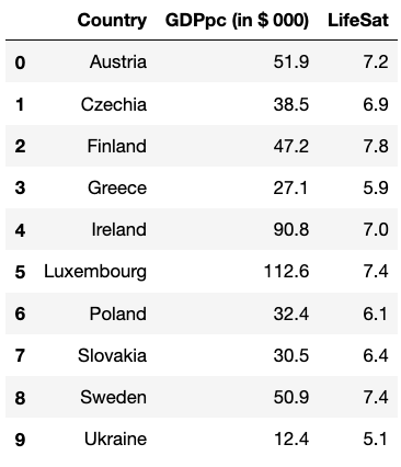
There are only 10 data points here, but the data are real! These are country average levels of life satisfaction and GDP per capita for a selection of countries in Europe in 2020.

I downloaded these data from the Our World in Data website for all of Europe, then randomly selected 10 countries. There are a lot of real-world studies on the topic of the relationship between wealth and happiness.

Here, we’ll focus on the concepts. We’ll get onto the Python code for regression later.

First, we can examine the relationship visually in a scatter plot:

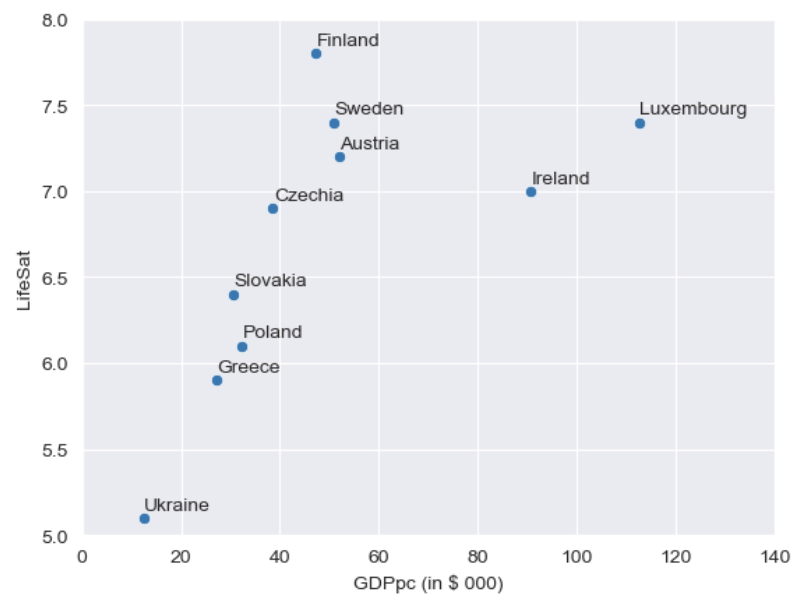
• What can you say about the relationship from eyeballing the scatter plot?

Click to reveal answer

There is a positive relationship

The correlation between life satisfaction and GDP per capita is 0.65 meaning, as you recall from topic 4, that there is a positive relationship of moderate strength. As GDP increases, so does average life satisfaction.

• The regression equation takes the form \(\hat{y}=a+bx\) where \(\hat{y}\) (known as “y-hat”) is the predicted value of \(y\), \(a\) is the intercept, and \(b\) is the slope. What are the \(y\) and \(x\) in the life satisfaction example?

Click to reveal answer

In our example, \(y\) is life satisfaction and \(x\) is GDP per capita

• In regression analysis, you need to be careful about saying which variable is \(y\) and which is \(x\). Why is this?

Click to reveal answer

In regression, we are always interested in the variables in terms of whether they are the outcome measure (i.e., the thing we are interested in explaining) or an explanatory variable (the thing that can explain our outcome measure). \(y\) is always the outcome measure, and \(x\) is always the explanatory variable.

Other terms to remember are dependent variable (\(y\)) and independent variable (\(x\)). We can have multiple independent variables in regression model, a point we will examine in detail next week.

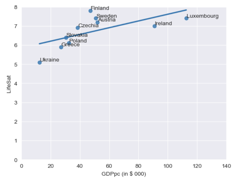
• So, let’s get to our regression equation for the life satisfaction data. We’ll get to the calculation later, so for now, I am just providing the regression equation for you. The regression equation here is Life Satisfaction= 5.85 + 0.018(GDPpc). Look back at the scatter plot, do the coefficients make sense?

Click to reveal answer

Yes! It becomes clearer when we add the line to the plot. We can see that the line crosses the \(y\)-axis at 5.85 so that makes sense. And eyeballing the slope, we can roughly see that life satisfaction increases from around 6.2 points to 6.9 points as GDP rises from 20 to 60 thousand (change in \(x\) = 40; 40*slope of 0.018 = 0.72). We’ll practise this more.

• One function of regression is that we can use it to “predict” the outcome variable of a hypothetical country. Imagine we want to know: what would be the predicted level of life satisfaction in a country with a GDP per capita of 150 thousand dollars (a very rich country!)? Plug in ‘150’ in place of \(x\) in the equation and find \(y\)-hat (just use a calculator, or excel, or pen and paper at this point).

Click to reveal answer

5.85 + (150*0.018) = life satisfaction of 8.55. (There are, of course, some assumptions here. We’ll talk about the assumptions of regression later in the course).

In the same way that we can plug in a hypothetical value (like 150 thousand dollars), we could also plug in the actual (or “observed”) values of \(x\) for our 10 countries. If we calculate y-hat for each country we can see the difference between the predicted level of life satisfaction and observed value. These have been added to the data table.

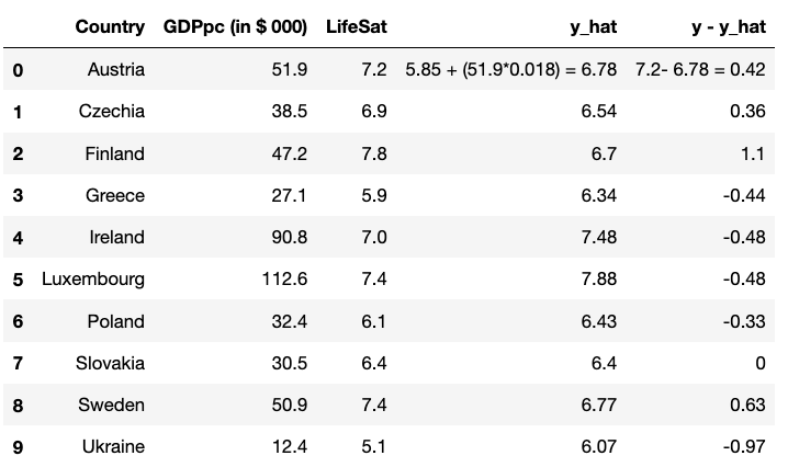
*What is the name for \(y\) minus \(\hat{y}\)?

Click to reveal answer

Residual

Looking at the residuals (\(y - \hat{y}\)), which are the largest values? (Take “largest” here to mean absolute values, i.e., both positive and negative numbers). How might you interpret those residuals?

Click to reveal answer

Finland has a positive residual of 1.10. Finland’s life satisfaction is 1.1 points higher than the regression line would predict based on GDP. Ukraine has a residual of -0.97 suggesting that life satisfaction is just under one point lower than predicted by the regression line.