
4.7. Spearman’s Rank Correlation#
Climate Example#
We will again use the a dataset containing carbon emissions, GDP and population for 164 countries (data from 2018).
These data came from Our World in Data, a fabulous Oxford-based organization that provides datasets and visualizations addressing global issues.
Set up Python libraries#
As usual, run the code cell below to import the relevant Python libraries
# Set-up Python libraries - you need to run this but you don't need to change it
import numpy as np
import matplotlib.pyplot as plt
import scipy.stats as stats
import pandas
import seaborn as sns
sns.set_theme() # use pretty defaults
Load and inspect the data#
Load the data from the file CO2vGDP.csv.
CO2vGDP = pandas.read_csv('https://raw.githubusercontent.com/jillxoreilly/StatsCourseBook/main/data/CO2vGDP.csv')
display(CO2vGDP)
| Country | CO2 | GDP | population | |
|---|---|---|---|---|
| 0 | Afghanistan | 0.2245 | 1934.555054 | 36686788 |
| 1 | Albania | 1.6422 | 11104.166020 | 2877019 |
| 2 | Algeria | 3.8241 | 14228.025390 | 41927008 |
| 3 | Angola | 0.7912 | 7771.441895 | 31273538 |
| 4 | Argentina | 4.0824 | 18556.382810 | 44413592 |
| ... | ... | ... | ... | ... |
| 159 | Venezuela | 4.1602 | 10709.950200 | 29825652 |
| 160 | Vietnam | 2.3415 | 6814.142090 | 94914328 |
| 161 | Yemen | 0.3503 | 2284.889893 | 30790514 |
| 162 | Zambia | 0.4215 | 3534.033691 | 17835898 |
| 163 | Zimbabwe | 0.8210 | 1611.405151 | 15052191 |
164 rows × 4 columns
We noted previously that our climate dataset is not suitable for a ‘normal’ Pearson’s correlation because it has one of the three freatures that violate the assumptions of Pearson’s correlation:
- Non-Straight-Line relationship between x and y
- Heteroscedasticity
- Outliers
In this case the problem was heteroscedasticity
Spearman’s Rank Correlation#
We therefore use a rank-based form of correlation called Spearman’s rank correlation coefficient $r_s$, which does not rely on the same assumptions as Pearson’s correlation.
$r_s$ can be calculated using the same built-in function pandas.df.corr():
CO2vGDP.corr(method='spearman')
---------------------------------------------------------------------------
ValueError                                Traceback (most recent call last)
Cell In[3], line 1
----> 1 CO2vGDP.corr(method='spearman')

File ~/opt/anaconda3/lib/python3.9/site-packages/pandas/core/frame.py:10054, in DataFrame.corr(self, method, min_periods, numeric_only)
  10052 cols = data.columns
  10053 idx = cols.copy()
> 10054 mat = data.to_numpy(dtype=float, na_value=np.nan, copy=False)
  10056 if method == "pearson":
  10057     correl = libalgos.nancorr(mat, minp=min_periods)

File ~/opt/anaconda3/lib/python3.9/site-packages/pandas/core/frame.py:1838, in DataFrame.to_numpy(self, dtype, copy, na_value)
   1836 if dtype is not None:
   1837     dtype = np.dtype(dtype)
-> 1838 result = self._mgr.as_array(dtype=dtype, copy=copy, na_value=na_value)
   1839 if result.dtype is not dtype:
   1840     result = np.array(result, dtype=dtype, copy=False)

File ~/opt/anaconda3/lib/python3.9/site-packages/pandas/core/internals/managers.py:1732, in BlockManager.as_array(self, dtype, copy, na_value)
   1730         arr.flags.writeable = False
   1731 else:
-> 1732     arr = self._interleave(dtype=dtype, na_value=na_value)
   1733     # The underlying data was copied within _interleave, so no need
   1734     # to further copy if copy=True or setting na_value
   1736 if na_value is not lib.no_default:

File ~/opt/anaconda3/lib/python3.9/site-packages/pandas/core/internals/managers.py:1794, in BlockManager._interleave(self, dtype, na_value)
   1792     else:
   1793         arr = blk.get_values(dtype)
-> 1794     result[rl.indexer] = arr
   1795     itemmask[rl.indexer] = 1
   1797 if not itemmask.all():

ValueError: could not convert string to float: 'Afghanistan'
The ‘methods’ available are:
- Pearson ('normal' correlation),
- Spearman (rank based) and
- Kendal (categorical; rarely used).
The default (the method used if no method is specified) is Pearson - we can see this by comparing the results with method specified as Pearson and no method specified:
CO2vGDP.corr(method='pearson')
| CO2 | GDP | population | |
|---|---|---|---|
| CO2 | 1.000000 | 0.795214 | -0.003745 |
| GDP | 0.795214 | 1.000000 | -0.054502 |
| population | -0.003745 | -0.054502 | 1.000000 |
CO2vGDP.corr()
| CO2 | GDP | population | |
|---|---|---|---|
| CO2 | 1.00000 | 0.79512 | -0.00019 |
| GDP | 0.79512 | 1.00000 | -0.02783 |
| population | -0.00019 | -0.02783 | 1.00000 |
The equation#
Let’s check our understanding by calculating Spearman’s correlation coefficient oursleves.
The equation is:
$$ r_s = 1 - 6 \sum{\frac{d^2}{n(n^2 - 1)}} $$
… where d is the difference in ranks between paired datapoints.
Let’s walk that through.
First, we create new columns containing the rank of each datapoint -
- the lowest GDP will have rank 1 and the highest will have rank 165
- the lowest CO2 emissions will have rank 1 and the highest will have rank 165
- the GDP aand CO2 ranks for each country need not match, but if GDP and CO2 are correlated,
- high-ranked countries for GDP should also be high-ranked for CO2
CO2vGDP['CO2_rank'] = CO2vGDP['CO2'].rank()
CO2vGDP['GDP_rank'] = CO2vGDP['GDP'].rank()

# We can see these most clearly if we sort the dataframe before displaying
display(CO2vGDP.sort_values(by='CO2'))
| Country | CO2 | GDP | population | CO2_rank | GDP_rank | |
|---|---|---|---|---|---|---|
| 39 | Democratic Republic of Congo | 0.0331 | 859.381714 | 87087352 | 1.0 | 4.0 |
| 26 | Central African Republic | 0.0471 | 623.488892 | 5094795 | 2.0 | 1.0 |
| 21 | Burundi | 0.0608 | 651.358887 | 11493476 | 3.0 | 2.0 |
| 27 | Chad | 0.0675 | 2046.363159 | 15604213 | 4.0 | 24.0 |
| 108 | Niger | 0.0830 | 964.660095 | 22577060 | 5.0 | 5.0 |
| ... | ... | ... | ... | ... | ... | ... |
| 128 | Saudi Arabia | 18.4541 | 50304.750000 | 35018132 | 160.0 | 154.0 |
| 9 | Bahrain | 20.7778 | 39498.765630 | 1487346 | 161.0 | 143.0 |
| 79 | Kuwait | 23.1008 | 65520.738280 | 4317190 | 162.0 | 160.0 |
| 148 | Trinidad and Tobago | 29.1223 | 28549.408200 | 1504707 | 163.0 | 128.0 |
| 122 | Qatar | 38.4397 | 153764.171900 | 2766743 | 164.0 | 164.0 |
164 rows × 6 columns
You can see that countries with low ranks for CO2 do tend to have low ranks for GDP.
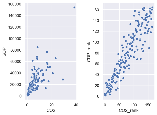
Let’s plot the data, and the ranked data, on scatterplots. You can see that the ranked data do not have the same heteroscedasticity issue as the data themselves.
plt.subplot(1,2,1)
sns.scatterplot(data=CO2vGDP, x='CO2', y='GDP')

plt.subplot(1,2,2)
sns.scatterplot(data=CO2vGDP, x='CO2_rank', y='GDP_rank')

plt.subplots_adjust(wspace = 0.5) # shift the plots sideways so they don't overlap
To continue the process of applying the equation, we make a new column containing the difference of ranks:
CO2vGDP['d'] = CO2vGDP['CO2_rank']-CO2vGDP['GDP_rank']
… and apply the formula:
n = len(CO2vGDP)

r_s = 1 - 6*sum(CO2vGDP['d']**2)/(n*(n**2 - 1))
print('r = ' + str(r_s))
r = 0.9143688871356087
Ta-daa! This should match the value from the built in function.
Spearman = Pearson on Ranks#
The equation for Spearman’s $r_s$ looks pretty weird, doesn’t it? What is that 6 doing there?!
I can’t tell you the derivation (although I believe I did once know it), but I can tell you a fun thing.
Spearman’s $r_s$ is exactly the same value as Pearson’s $r$ claculated on the ranks.
Let’s try it!
# make a new dataframe with only ranks
CO2vGDP_ranks = CO2vGDP[['CO2_rank','GDP_rank']]
display(CO2vGDP_ranks)
| CO2_rank | GDP_rank | |
|---|---|---|
| 0 | 16.0 | 22.0 |
| 1 | 58.0 | 73.0 |
| 2 | 94.0 | 93.0 |
| 3 | 41.0 | 59.0 |
| 4 | 99.0 | 105.0 |
| ... | ... | ... |
| 160 | 77.0 | 55.0 |
| 161 | 106.0 | 96.0 |
| 162 | 24.0 | 26.0 |
| 163 | 29.0 | 36.0 |
| 164 | 44.0 | 14.0 |
165 rows × 2 columns
# Calculate **Pearson's** correlation on the ranks
CO2vGDP_ranks.corr(method='pearson')
| CO2_rank | GDP_rank | |
|---|---|---|
| CO2_rank | 1.000000 | 0.913841 |
| GDP_rank | 0.913841 | 1.000000 |
Yep, the correlation is 0.9138 - the exact same value as $r_s$