2.7. Grouping data

In many datasets, data can be categorized and we would wish to give descriptive statistics separately for each category.

Set up Python libraries

As usual, run the code cell below to import the relevant Python libraries

# Set-up Python libraries - you need to run this but you don't need to change it
import numpy as np
import matplotlib.pyplot as plt
import scipy.stats as stats
import pandas 
import seaborn as sns
sns.set_theme()

Load and view the data

Let’s load the datafile “vehicles.csv” which contains size data on vehicles parked at a vehicle-ferry terminal at 1pm on Sunday 24th April 2022, which they regard as a representative sample.

vehicles = pandas.read_csv('https://raw.githubusercontent.com/jillxoreilly/StatsCourseBook/main/data/vehicles.csv')
display(vehicles)

	length	height	width	type
0	3.9187	1.5320	1.8030	car
1	4.6486	1.5936	1.6463	car
2	3.5785	1.5447	1.7140	car
3	3.5563	1.5549	1.7331	car
4	4.0321	1.5069	1.7320	car
...	...	...	...	...
1359	15.5000	4.2065	2.5112	truck
1360	14.4960	4.1965	2.5166	truck
1361	15.9890	4.1964	2.4757	truck
1362	14.3700	4.2009	2.5047	truck
1363	14.2350	4.2016	2.5212	truck

1364 rows × 4 columns

That was a long list of vehicles!

• What information do we have about each vehicle?

Obtain descriptive statistics

We can use the built in functions in pandas.describe() to return descriptives for our data

vehicles['length'].describe()

count    1364.000000
mean        6.722972
std         4.232075
min         3.110900
25%         3.929450
50%         4.419300
75%         9.260325
max        16.231000
Name: length, dtype: float64

Why group the data?

You can see above that the mean length of vehicles in the car park is 6.72m.

This is surprising as it is rather longer than even a large family car

To get a better sense of the length data, I am going to plot them.

Don’t worry too much about the plotting code for now, as there are dedicated exercises on plotting later.

sns.histplot(data=vehicles, x="length",  bins = np.arange(0,16,0.5))
plt.xlabel('vehicle length (m)')

Text(0.5, 0, 'vehicle length (m)')

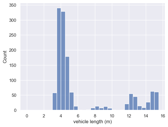
Interesting. It looks like there are several clusters of vehicle lengths.

Have a look back at our dataframe - is there some information there that could explain the different clusters?

• Probably the clusters relate to different vehicle types

I can plot vehicle types in different colours (again no need ot worry about the plotting code at this stage)

sns.histplot(data=vehicles, x="length", bins = np.arange(0,16,0.5), hue="type")
plt.xlabel('vehicle length (m)')

Text(0.5, 0, 'vehicle length (m)')

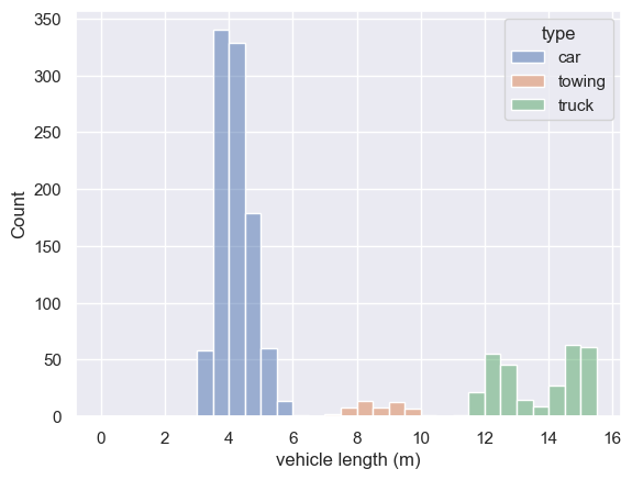
Aha. We might want to describe our data separately for each by vehicle type.

Grouping into separate dataframes

One way to do this is to create separate dataframes for each vehicle type:

cars = vehicles[vehicles['type']=='car']
cars.describe()

	length	height	width
count	981.000000	981.000000	981.000000
mean	4.197994	1.580810	1.791925
std	0.517761	0.059263	0.046921
min	3.110900	1.430400	1.624100
25%	3.815400	1.540000	1.760200
50%	4.121600	1.574500	1.790400
75%	4.518400	1.611900	1.820900
max	6.102400	1.899300	1.958000

we can see that 981 of the vehicles were cars, and their mean length was 4.198m, much shorter than the mean over all vehicles.

Try modifying the code below to get descriptive statistics for trucks:

# modify the code to get descritives for trucks
cars = vehicles[vehicles['type']=='car']
cars.describe()

	length	height	width
count	981.000000	981.000000	981.000000
mean	4.197994	1.580810	1.791925
std	0.517761	0.059263	0.046921
min	3.110900	1.430400	1.624100
25%	3.815400	1.540000	1.760200
50%	4.121600	1.574500	1.790400
75%	4.518400	1.611900	1.820900
max	6.102400	1.899300	1.958000

pandas.groupby

We can also use the pandas function groupby to split up our dataframe according to a categorical variable, in this case vehicle type.

vehicles.groupby(['type']).describe()

	length								height					width
	count	mean	std	min	25%	50%	75%	max	count	mean	...	75%	max	count	mean	std	min	25%	50%	75%	max
type
car	981.0	4.197994	0.517761	3.1109	3.8154	4.1216	4.5184	6.1024	981.0	1.580810	...	1.6119	1.8993	981.0	1.791925	0.046921	1.6241	1.7602	1.79040	1.82090	1.9580
towing	53.0	8.672951	0.713460	7.2561	8.1323	8.6894	9.2191	10.0980	53.0	2.897838	...	2.9064	2.9445	53.0	2.248326	0.008222	2.2292	2.2442	2.24790	2.25400	2.2642
truck	330.0	13.915864	1.343028	11.1480	12.5640	14.3650	15.0750	16.2310	330.0	4.072725	...	4.2009	4.2137	330.0	2.501304	0.015871	2.4629	2.4898	2.50145	2.51155	2.5467

3 rows × 24 columns

Yikes, that was an unweildy table!

It may be preferable to output descriptives only for one measure (eg length):

vehicles.groupby(['type'])['length'].describe()

	count	mean	std	min	25%	50%	75%	max
type
car	981.0	4.197994	0.517761	3.1109	3.8154	4.1216	4.5184	6.1024
towing	53.0	8.672951	0.713460	7.2561	8.1323	8.6894	9.2191	10.0980
truck	330.0	13.915864	1.343028	11.1480	12.5640	14.3650	15.0750	16.2310

… or to output one descriptive (such as the mean) at a time, rather than the whole table

vehicles.groupby(['type']).mean()

	length	height	width
type
car	4.197994	1.580810	1.791925
towing	8.672951	2.897838	2.248326
truck	13.915864	4.072725	2.501304