
2.11. Tutorial Exercises II - optional#
In this section we use our skills in creating for loops to investigate the properties of the mean and standard deviation
This material will not be assessed but is presented for your interest and understanding (and to practice some coding!)
You should only tackle it if you have plenty of time left in the tutorial after completing Tutorial Exercises I.
This exercise involves more coding than the rest of the exercises this week - in particular it involves for loops. You may want to review the material in chapter 1, ‘preparatory work’ to help you with this. If you didn’t get to do the ‘preparatory work’ yet, maybe just do that instead.
Why $(n-1)$?#
In the exercises and lecture this week, we calculated the mean and standard deviation of data.
A casual description of the variance ($s^2$, standard deviation squared) is that it is approximately the average squared deviation between datapoints and the mean - therefore to calculate it we:
- calculate the difference between each data point and the mean
- square those differences
- add them all up
- divide by the number of datapoints
That would suggest the following formula:
(1)
$$ s^2 = \sum{\frac{{(x_i - \bar{x})}^2}{n}} $$
But in fact the formula has $(n-1)$ on the bottom:
(2)
$$ s^2 = \sum{\frac{{(x_i - \bar{x})}^2}{n-1}} $$
Why? To understand this we first need to introduce the concept of estimators
Introducing estimators#
Typically, our dataset is a sample from a larger population and we want to use the mean and sd not so much to describe our sample, as to describe the (likely) properties of the population from which they are drawn.
The mean and sd as we have been calculating them are actually estimators of the population mean and sd (based on the sample) - not a straight description of the sample.

To illustrate the difference between the sd of the sample itself, and the sd of the population as estimated from the sample:
Say we measure the height of 10 men (this is a sample from a larger population with 20 million members). We are really interested in the characteristics of the population (the group of 20 million) - not just the 10 we happened to pick for our sample.
- To describe the sample, we calculate the mean of the sample and the spread (sd) of the sample members about the sample mean
- To describe the underlying population, we estimate the population mean, and estimate the spread (sd) of population members about the population mean
In case (2), we will use the sample mean and sample sd to help us estimate the population mean and population sd.
Let’s use simulation to find out what happens if we try to estimate the population standard deviation using the two different possible equations above, with either $n$ or $n-1$ on the bottom.
Demonstration by Simulation#
Set up Python libraries#
As usual, run the code cell below to import the relevant Python libraries
# Set-up Python libraries - you need to run this but you don't need to change it
import numpy as np
import matplotlib.pyplot as plt
import scipy.stats as stats
import pandas
import seaborn as sns
sns.set_theme()
Population data#
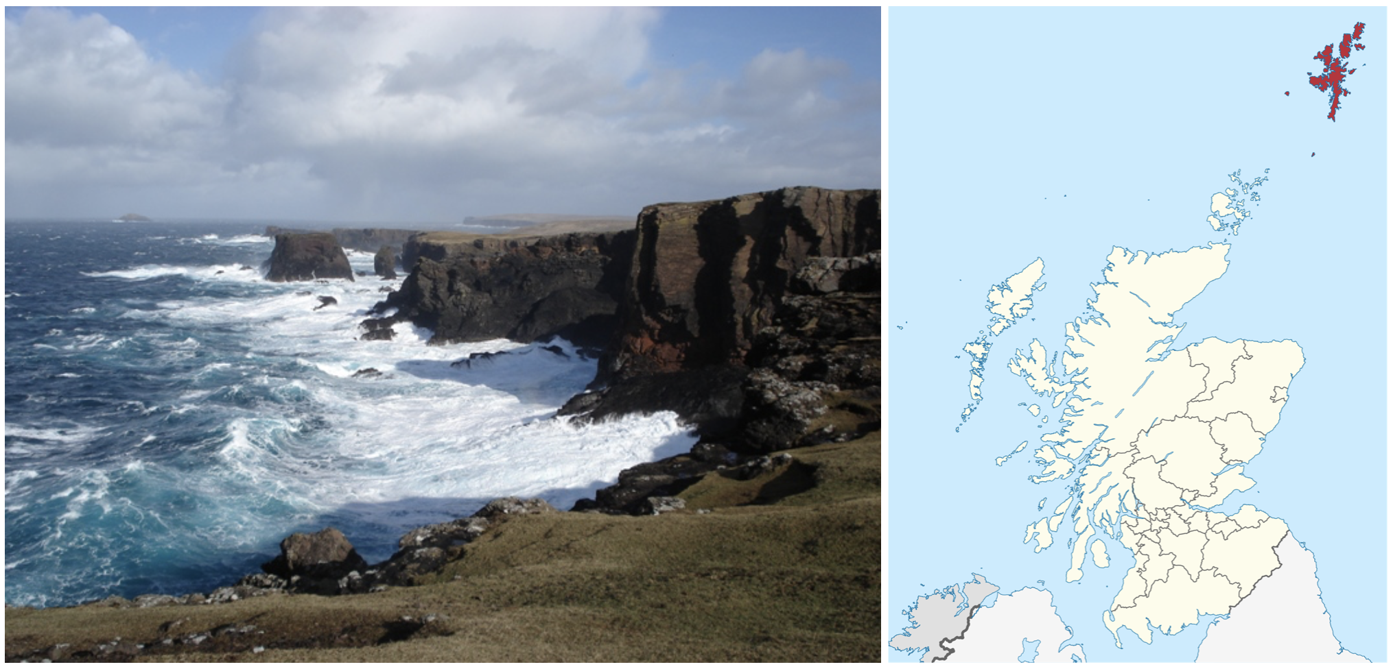
Let’s imagine that our population is all the men on the island of Shetland - about 10,000 people
I’m going to create a numpy array of 10,000 heights (these are simulated data but you could do this with real data from a survey if you had them)
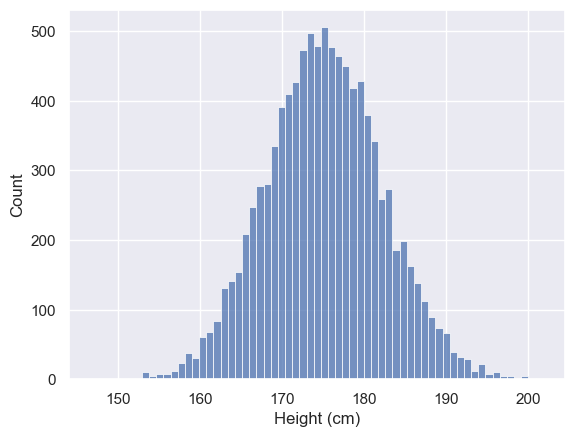
popHeights = np.random.normal(175,7,10000)

# Let's plot them
sns.histplot(popHeights)
plt.xlabel('Height (cm)')
Text(0.5, 0, 'Height (cm)')
Since we have the whole population dataset here, we can work out the population mean and standard deviation directly:
mPop = popHeights.mean()
sdPop = popHeights.std()
print('population mean = ' + str(mPop))
print('population sd = ' + str(sdPop))
population mean = 175.1094178266492
population sd = 7.10851500877297
Sample data#
Now let’s imagine that we don’t have access to the heights of every single man in the population of Shetland, but instead we measure a random sample of 10 men.
We can simulate this by picking 10 values at random from our array of population heights (which is a virtual version of picking 10 random men off the street in Shetland) using the function np.random
# let's call our sample 'x'
x = np.random.choice(popHeights, 10, replace=False)
print(x)
[168.50114151 172.94474047 156.02052468 171.88053982 167.40166564
 183.55056417 175.40347142 174.9195068  185.02639425 174.84473845]
Let’s calculate the mean and standard deviation of the sample - because we are going to try out different equations, we will not use the built in functions mean and std but instead enter the equations ourselves.
Remember that the symbol ** means ‘power’ - so 3**2 means $3^2$
Remember also that $n^\frac{1}{2} = \sqrt{n}$ so for example 4**0.5 = $\sqrt{4}$ = 2
n=10
x = np.random.choice(popHeights, n, replace=False)

# if you are stuck you can find the answer at the bottom of the page
m = # your code here for the mean
s1 = # your code here for the s.d. with n on the bottom
s2 = # your code here for the s.d. with n-1 on the bottom

print('mean = ' + str(m))
print('sd (with n on the bottom) = ' + str(s1))
print('sd (with n-1 on the bottom) = ' + str(s2))
  Cell In[5], line 5
    m = # your code here for the mean
        ^
SyntaxError: invalid syntax
If you run the cell above a few times you will notice a couple of things:
- The value for sd with n on the bottom is always lower
- The estimates of the mean and sd are pretty variable across samples!
Simulate many samples#
To establish which equation for the sd gives a better match for the population sd (calculated from the whole population of 10,000 men), we are going to need to draw a lot of samples and get the average value for the standard deviation:
nSamples = 1000
# create empty arrays to store the result of the simulation
m = np.empty(nSamples)
s1 = np.empty(nSamples)
s2 = np.empty(nSamples)
n = 10

for i in range(....):
    # build the loop yourself!
    # if you are stuck you can find the answer at the bottom of the page


# print the results of the simulation
print('mean value of the mean is ' + str(np.mean(m)))
print('mean value of sd with n on the bottom is ' + str(np.mean(s1)))
print('mean value of sd with n-1 on the bottom is ' + str(np.mean(s2)))
print(' ') # blank line

# and a reminder:
mPop = popHeights.mean()
sdPop = popHeights.std()
print('population mean = ' + str(mPop))
print('population sd = ' + str(sdPop))
mean value of the mean is 174.87163049278854
mean value of sd with n on the bottom is 6.474290353743315
mean value of sd with n-1 on the bottom is 6.82450125036204

population mean = 174.88960457679235
population sd = 7.005912927563505
It looks like the version with $n-1$ gets us closer to the the true standard deviation (although it is still not perfect).
Check your understanding of the code#
- What is stored in s1 and s2.
- What does the line s1 = np.empty(nSamples) do and why is it necessary?
- What was popHeights again?
Justifying $n-1$#
If we calculate the standard deviation of the sample as we might naively (with $n$ rather than $n-1$ on the bottom), we would systematically underestimate the standard deviation of the population. This bias is worse when the sample size is small.
To get a sense why this is, look at the diagram below.
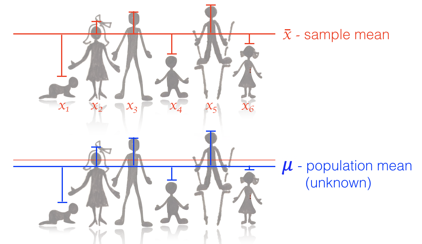
When calculating the standard deviation from our sample, we look at the deviations of the datapoints about our estimate of the mean, $\bar{x}$.
Now, $\bar{x}$ is calculated from the sample itself (and as it happens, the formula for the mean minimizes the squared devations $\sum{{(x_i - \bar{x})}^2}$) - so there is no possible value of the mean that could result in a lower set of deviations.
Therefore if we knew the true population mean $\mu$ (which is similar to $\bar{x}$ but won’t be exactly the same), and could calculate the deviations about it $\sum{(x_i - \mu)^2}$ we would certainly get a higher value for the standard deviation.
The reason the bias is worse for smaller samples is because the value of $\bar{s}$ is more swayed by the particular values in the sample $x$ when $n$ is small.
Vary sample size#
To examine the claim that the underestimation of the population standard deviation is worse when $n$ is small (for the sd formula with $n$ on the bottom), lets try simulating samples with different values of n.
This is a double loop - I’m not expecting you to build this yourself but if you are keen you could try to follow through the logic:
nSamples = 1000
# create empty arrays to store the result of the simulation each of nSamples
m = np.empty(nSamples)
s1 = np.empty(nSamples)
s2 = np.empty(nSamples)

# values of n to try
nVals = [2,5,10,20,50,100]
# create some more empty arrays to store the average values
# of m, s1, s2 for each value of n that we will try
m_n = np.empty(len(nVals))
s1_n = np.empty(len(nVals))
s2_n = np.empty(len(nVals))


for j in range(len(nVals)):
    n=nVals[j]
    for i in range(nSamples):
        x = np.random.choice(popHeights, n, replace=False)
        m[i] = sum(x)/n
        s1[i] = (sum((x - m[i])**2)/n)**0.5
        s2[i] = (sum((x - m[i])**2)/(n-1))**0.5

    m_n[j] = np.mean(m)
    s1_n[j] = np.mean(s1)
    s2_n[j] = np.mean(s2)


# Plot the results
# Don't worry about this - we are covering plotting next week
plt.figure
plt.plot(nVals,s1_n,'b.-')
plt.plot(nVals,s2_n,'r.-')
plt.axhline(y = popHeights.std(), color='k', linestyle=':') # plot the actual population sd as lback dotted line
plt.xlabel('$n$')
plt.ylabel('estimated pop. standard deviation')
plt.legend(['using $n$','using $n-1$','actual population sd'])
<matplotlib.legend.Legend at 0x7fa8e2b38ee0>
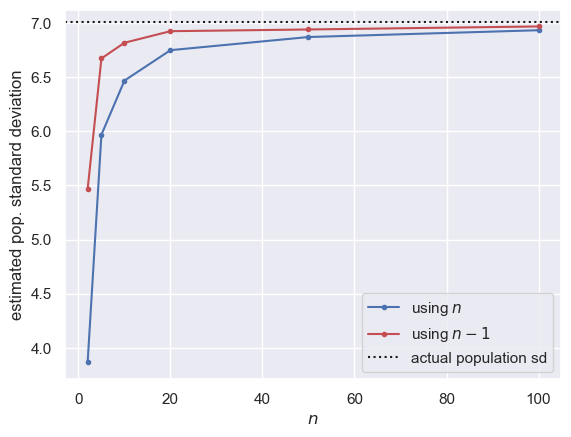
We can see that:
- the underestimation bias is greater for smaller sample size
- the bias is reduced, but not eliminated, for the $n-1$ version
In fact there is no simple solution to correct the bias completely when estimating the population standard deviation.
Hints#
Here are the missing bits of code - you are welcome to copy-paste them but once you have, I’d suggest trying to work through them (with your tutor if helpful) and then try to recreate from memory as in coding, you learn by doing.
# formulae for mean and standard deviation
m = sum(x)/n # mean
s1 = (sum((x - m)**2)/n)**0.5 # s.d. with n on the bottom
s2 = (sum((x - m)**2)/(n-1))**0.5 # s.d. with n-1 on the bottom
# for loop to try 1000 samples of size n

nSamples = 1000
# create empty arrays to store the result of the simulation
m = np.empty(nSamples)
s1 = np.empty(nSamples)
s2 = np.empty(nSamples)
n = 10

for i in range(nSamples):
    x = np.random.choice(popHeights, n, replace=False)
    m[i] = sum(x)/n
    s1[i] = (sum((x - m[i])**2)/n)**0.5
    s2[i] = (sum((x - m[i])**2)/(n-1))**0.5