3.3. Histogram

If we want to see the shape of a data distribution, the histgram can be a good choice

In this section we will see how to plot a histogram using Python and what choices we can make to show the data distribution clearly and accurately

We will also consider some of the limitations of the histogram for small datasets. In the next section we meet a related plot, the Kernel Density Estimate plot, which can mitigate these limitations.

Example

We will look at a small sample of height data for brother-sister pairs.

Set up Python libraries

As usual, run the code cell below to import the relevant Python libraries

# Set-up Python libraries - you need to run this but you don't need to change it
import numpy as np
import matplotlib.pyplot as plt
import scipy.stats as stats
import pandas 
import seaborn as sns
sns.set_theme() # use pretty defaults

Load and inspect the data

Load the file brotherSisterData.csv which contains heights in cm for 25 brother-sister pairs

heightData = pandas.read_csv('https://raw.githubusercontent.com/jillxoreilly/StatsCourseBook/main/data/BrotherSisterData.csv')
display(heightData)

	brother	sister
0	174	172
1	183	180
2	154	148
3	172	180
4	172	165
5	161	159
6	167	159
7	172	164
8	195	188
9	189	175
10	161	160
11	181	177
12	175	168
13	170	169
14	175	165
15	169	164
16	169	163
17	180	176
18	180	176
19	180	172
20	175	170
21	162	157
22	175	172
23	181	179
24	173	171

In this section, we are going to focus just on the brothers.

Plot a histogram

Let’s start by plotting a histogram of the data to see what the distriubtion of heights is.

In this course we will use plotting functions from the libraries matplotlib (imported as plt) and seaborn (imported as sns).

Therefore all the plotting commands will be preceded by either plt. or sns.

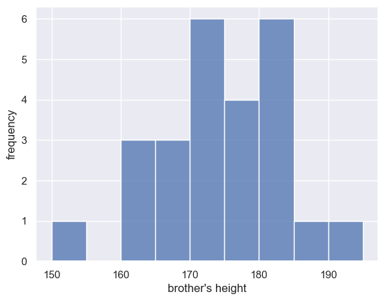
sns.histplot(heightData["brother"],  bins = range(150,200,5), color='b')
plt.xlabel('brother\'s height') 
plt.ylabel('frequency')

Text(0, 0.5, 'frequency')

Bin size

In a histogram, we bin data (in this case, we group the heights into 5cm-wide bins), and count how many data values fall in each bin

I used bins of 5cm to group the heights, and used x-axis values from 150 to 200 cm.

• Can you find where in the code this is specified?
• In the code block below, change the width of the bins to 1cm. What do you notice? Can you see the shape of the distribution better or worse using the 1cm bins?

sns.histplot(heightData["brother"],  bins = range(150,200,5), color='b') # hint - the numbers 150, 200 and 5 are the minimum/maximum x axis values and the bin size
plt.xlabel('brother\'s height') 
plt.ylabel('frequency')

Text(0, 0.5, 'frequency')

Bin boundaries

One problem with using a histogram when you have only a small number of data points is that the shape of the histogram can depend a lot on where the bin boundaries happen to fall.

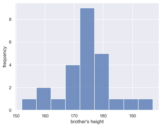
Look at the following plot of brothers’ heights, again grouped into 5cm bins but with different bin boundaries:

Exercises

• What change in the code moved the bin boundaries?
• What were the old bin boundaries? What are the new bin boundaries?
• Edit the code so that the in boundaries are at 153,158,163 etc

sns.histplot(heightData["brother"],  bins = range(152,202,5), color='b')
plt.xlabel('brother\'s height') 
plt.ylabel('frequency')

Text(0, 0.5, 'frequency')

The shape of the distribution looks quite different!

We can see this more clearly if we plot both versions next to each other (this is achieved using the command subplot - we will revisit it later so don’t worry too much about that)

plt.subplot(1,2,1)
sns.histplot(heightData["brother"],  bins = range(150,200,5), color='b')
plt.xlabel('brother\'s height') 
plt.ylabel('frequency')
plt.ylim((0,10)) # this sets the y axis limits rather than letting the computer choose them automatically

plt.subplot(1,2,2)
sns.histplot(heightData["brother"],  bins = range(152,202,5), color='b') 
plt.xlabel('brother\'s height') 
plt.ylabel('frequency')
plt.ylim((0,10))

plt.subplots_adjust(wspace = 0.5) # shift the plots sideways so they don't overlap

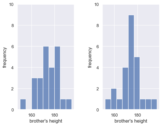
Originally (left) the bin boundaries were at 150cm, 155cm, 160cm etc.

In the second histogram (right) the bin boundaries were at 152cm, 157cm, 162cm etc.

Moving the bin boundaries changed how many observations fell in each bin and thus the shape of the histogram. This can happen easily when you have a small number of observations in each bin (check the y-axis in the above histogram - you can see that moving just one observation makes a big difference to the height of the bars).

For this reason, a histogram may not be the best representation of the data for a small sample.

Exercises

• I added a line of code to set the y axis limits to be [0,10] - why do you think I did this?
• Try removing or commenting it out and see how the two histograms change - is it easier to compare with fixed or automatic y-axis?