11.9. The Wilcoxon Sign-Rank Test

The t-test is valid only when the data within each group (for independent samples t-test) or the pairwise differences (for paired samples t-test) are Normally distributed

As we have seen in the lecture, many real life data distributions are normal, but many others are not.

For non-Normal data we can use non-parametric tests, which do not assume that the data are drawn from a Normal distribution.

The Wilcoxon Sign-Rank Test is a test for paired samples. It tests whether the median difference between the members of each pair is greater than zero. As such it is often considered to be a non-parametric equivalent for the paired samples t-test.

The Wilcoxon Sign-rank test is not the same as the Wilcoxon Rank Sum test (Mann Whitney U test) which is for independent samples

We will us a Python function called wilcoxon from the scipy.stats package to run the test

Set up Python libraries

As usual, run the code cell below to import the relevant Python libraries

# Set-up Python libraries - you need to run this but you don't need to change it
import numpy as np
import matplotlib.pyplot as plt
import scipy.stats as stats
import pandas 
import seaborn as sns

Example: the Sign-Rank Test

It has been argued that birth order in families affects how independent individuals are as adults - either that first-born children tend to be more independent than later born children or vice versa.

In a (fictional!) study, a researcher identified 20 sibling pairs, each comprising a first- and second- born child from a two-child family. The participants were young adults; each participant was interviewed at the age of 21.

The researcher scored independence for each participant, using a 25 point scale where a higher score means the person is more independent, based on a structured interview.

Carry out a statistical test for a difference in independence scores between the first- and second-born children.

Note that this is a paired samples design - each member of one group (the first-borns) has a paired member of the other group (second-borns).

Inspect the data

The data are provided in a text (.csv) file.

Let’s load the data as a Pandas dataframe, and plot them to get a sense for their distribution (is it normal?) and any outliers

# load the data and have a look
pandas.read_csv('https://raw.githubusercontent.com/jillxoreilly/StatsCourseBook/main/data/BirthOrderIndependence.csv')

	FirstBorn	SecondBorn
0	12	10
1	18	12
2	13	15
3	17	13
4	8	9
5	15	12
6	16	13
7	5	8
8	8	10
9	12	8
10	13	8
11	5	9
12	14	8
13	20	10
14	19	14
15	17	11
16	2	7
17	5	7
18	15	13
19	18	12

Scatterplot

In the case of paired data, the most effective way to get a sense of the data is a scatterplot:

birthOrder = pandas.read_csv('https://raw.githubusercontent.com/jillxoreilly/StatsCourseBook/main/data/BirthOrderIndependence.csv')

plt.scatter(data = birthOrder, x="FirstBorn", y="SecondBorn")
plt.xlabel("independence: first born")
plt.ylabel("independence: second born")

# add the line x=y (ie a line from point(50,50) to (110,110)) for reference 
plt.plot([0,20],[0,20],'r--')

[<matplotlib.lines.Line2D at 0x7fc94013b580>]

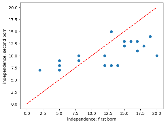
Comments:

• There is some correlation in independeence between first- and second-borns (independent first borns have independent second-born siblings)
• There are slightly more sibling pairs where the first-born is the more independent (points lying below the line x=y)
• It looks like in families with higher independence scores, the first-born is more indepenent than the second-born but for families with lower independednce scores, the opposite is true

Check assumption of normality

In the case of paired data, the assumption we would need to meet to use a t-test is that the differences between conditions (for each participant) are normally distributed - let’s add a column to our pandas data frame to contain the differences

birthOrder['Diff'] = birthOrder.FirstBorn - birthOrder.SecondBorn
birthOrder

	FirstBorn	SecondBorn	Diff
0	12	10	2
1	18	12	6
2	13	15	-2
3	17	13	4
4	8	9	-1
5	15	12	3
6	16	13	3
7	5	8	-3
8	8	10	-2
9	12	8	4
10	13	8	5
11	5	9	-4
12	14	8	6
13	20	10	10
14	19	14	5
15	17	11	6
16	2	7	-5
17	5	7	-2
18	15	13	2
19	18	12	6

Now let’s plot the differences to get a sense of whether they are normally distributed.

sns.kdeplot(birthOrder["Diff"],  color='b', shade=True)
sns.rugplot(birthOrder["Diff"], height=0.1, color='b')

/var/folders/q4/twg1yll54y142rc02m5wwbt40000gr/T/ipykernel_3474/4070573100.py:1: FutureWarning: 

`shade` is now deprecated in favor of `fill`; setting `fill=True`.
This will become an error in seaborn v0.14.0; please update your code.

  sns.kdeplot(birthOrder["Diff"],  color='b', shade=True)

<Axes: xlabel='Diff', ylabel='Density'>

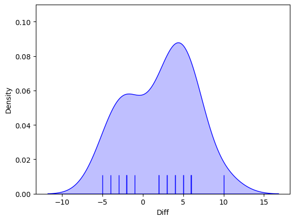
The distribution does not look very Normal, with a hint of bimodality (two peaks).

Since there is also no theoretical reason to think the differences should be normally distributed, we will use a non-parametric test

Hypotheses

Ho: the median difference in independence between first- and second-born siblings is is zero

Ha: the median difference in independence is not zero

This is a two-tailed test as the researcher’s hypothesis (described above) is not directional.

We will test at the $\alpha = 0.05$ significance level

Descriptive statistics

We obtain the relevant descriptive statistics. For the t-test we reported the summary statistics (mean, s.d. and $n$) that went into the formula for $t$. The same approach won’t quite work here as the test is not based on summary statistics. However, common sense suggests that reporting the median for each group, a measure of spread based on ranks (namely the IQR), and the sample size would give the reader an idea of the data.

birthOrder.describe()

	FirstBorn	SecondBorn	Diff
count	20.000000	20.000000	20.000000
mean	12.600000	10.450000	2.150000
std	5.364601	2.438183	4.120232
min	2.000000	7.000000	-5.000000
25%	8.000000	8.000000	-2.000000
50%	13.500000	10.000000	3.000000
75%	17.000000	12.250000	5.250000
max	20.000000	15.000000	10.000000

Carry out the test

We carry out the test using the function wilcoxon from scipy.stats, here loaded as stats

stats.wilcoxon(birthOrder['FirstBorn'],birthOrder['SecondBorn'],alternative='two-sided')
#help(stats.wilcoxon)

WilcoxonResult(statistic=46.0, pvalue=0.026641845703125)

The inputs to stats.wilcoxon are:

• the two samples to be compared (the values of FirstBorn and SecondBorn from our Pandas data frame birthOrder)
• the argument alternative='greater', which tells the computer to run a one tailed test that mean of the first input (FirstBorn) is greater than the second (SecondBorn).

The outputs are a value of the test statistic ($T=164$) and pvalue ($p=0.0133$) - if this is less than our $\alpha$ value 0.5, there is a significant difference.

More explanation of how T is calculated below.

Draw conclusions

As the p value of 0.0133 is less than our alpha value of 0.05, the test is significant.

We can conclude that the median difference in idenpendence is positive, ie the first borns are more independent

11.10. How the Wilcoxon Sign-Rank test works

You have seen how to carry out the Sign-Rank test using scipy.stats but you may be none the wiser about how the computer arrived at the test statistic and p value.

In this section we will build our own version of the test step by step to understand how it worked.

How to do the test (if you were doing it with pencil and paper)

1. Obtain the difference (in independence score) for each pair

2. Rank the differences regardless of sign (e.g. a difference of +4 is greater than a difference of -3, which is greater than a difference of +2). Remove pairs with zero difference

3. Calculate the sum of ranks assigned to pairs with a positive difference (first-born more independent than second-born) - this is $R+$

4. Calculate the sum of ranks assigned to pairs with a negative difference (first-born more independent than second-born) - this is $R-$

5. The test statistic $T$ is either:

   • $R+$ if we expect positive differences to have the larger ranks (in this case, that equates to expecting first-borns to have higher scores)

   • $R-$ if we expect negative differences to have the larger ranks (in this case, that equates to expecting second-borns to have higher scores)

   • The smaller of $R+$ and $R-$ for a two tailed test (as in the example, we have no a-prior hypothesis about direction of effect)

6. $T$ is compared with a null distribution (the expected distribubtion of $T$ obtained in samples drawn from a population in which there is no true difference between groups)

Step 1: Obtain the differences

We already did this and added a column ‘Rank’ do our dataframe

Step 2: Rank the differences regardless of sign

We can obtain the absolute differences and save them in a new column of the dataframe as follows

birthOrder['AbsDiff'] = birthOrder['Diff'].abs()
birthOrder

	FirstBorn	SecondBorn	Diff	AbsDiff
0	12	10	2	2
1	18	12	6	6
2	13	15	-2	2
3	17	13	4	4
4	8	9	-1	1
5	15	12	3	3
6	16	13	3	3
7	5	8	-3	3
8	8	10	-2	2
9	12	8	4	4
10	13	8	5	5
11	5	9	-4	4
12	14	8	6	6
13	20	10	10	10
14	19	14	5	5
15	17	11	6	6
16	2	7	-5	5
17	5	7	-2	2
18	15	13	2	2
19	18	12	6	6

Then we rank the absolute differences

birthOrder['Rank'] = birthOrder['AbsDiff'].rank()
birthOrder

	FirstBorn	SecondBorn	Diff	AbsDiff	Rank
0	12	10	2	2	4.0
1	18	12	6	6	17.5
2	13	15	-2	2	4.0
3	17	13	4	4	11.0
4	8	9	-1	1	1.0
5	15	12	3	3	8.0
6	16	13	3	3	8.0
7	5	8	-3	3	8.0
8	8	10	-2	2	4.0
9	12	8	4	4	11.0
10	13	8	5	5	14.0
11	5	9	-4	4	11.0
12	14	8	6	6	17.5
13	20	10	10	10	20.0
14	19	14	5	5	14.0
15	17	11	6	6	17.5
16	2	7	-5	5	14.0
17	5	7	-2	2	4.0
18	15	13	2	2	4.0
19	18	12	6	6	17.5

… phew! Let’s just check in on our understanding:

• In the largest ranked pair (rank 20), the difference is +10 (the first-born's independence score was 10 points higher than the second-born's).
• Several pairs with a difference of 4 points between siblings share rank 11. In some of these pairs the first-orn was more independent, in some pairs the second-born was more independent.
  • Find them in the table.
• In 13/20 pairs the first-born was more independent; in 7/20 pairs the second-born was more independent.

Work out the test-statistic $T$

We need to add up all the ranks assigned to pairs with positive differences (first-born is more independent) to get $R+$ and all the ranks assigned to pairs with negative differences (second-born is more independent) to get $R-$

Rplus = sum(birthOrder.loc[(birthOrder['Diff']>0), 'Rank'])
Rminus = sum(birthOrder.loc[(birthOrder['Diff']<0), 'Rank'])

print('R+ = ' + str(Rplus))
print('R- = ' + str(Rminus))

R+ = 164.0
R- = 46.0

T is the smaller of these - you might like to check that the value obtained below matches the ‘test statistic’ from the function scipy.stats.wilcoxon that we used above

T = min(Rplus, Rminus)
print('T = ' + str(T))

T = 46.0

Establish the null distriubtion

To convert our $T$ to a $p$-value, we need to know how the probability of obtaining that value of $T$ due to chance if the null hypothesis were true.

What do we mean by “If the null were true”?

If the null were true, the first- and second-born siblings should be equally likely to be more independent. If this were true, high- and low-ranked differences would occur randomly in favour of the first-born and second-born sibling. So each rank (in this case, the ranks 1-20, as we have 20 sibling pairs) might equally likely feed into $R+$ or $R-$

Estalbishing the null by complete enumeration

For a much smaller sample size, we could work out all the possible ways the ranks could be randomly assigned to contribute to $R+$ or $R-$, and work out in what proportion of cases this simulated $U$ was as large as, or larger than, the value of $U$ from our experiment.

This is not practical for larger samples as there are too many possible ways to deal the ranks (too many combbinations). In the example above where $n_1 = 9$ and $n_2 = 11$, the number of possible deals or combinations is 167960 - for larger $n$ the number of combinations becomes astronomical.

Establishing the null by simulation

We can work out the null approximately by doing a lot of random ‘deals’ of the ranks to $R+$ or $R-$, calculating $T$ for each case, and work out in what proportion of cases this simulated $T$ was as large as, or larger than, the value of $T$ from our experiment.

“A lot” might be 10,000 or more (this is still much lower than the number of possible deals under complete enumeration)

Let’s try it!

# Possible ranks are the numbers 1 to 20 (remember Python uses the counterintuitive syntax [1,21))
ranks = np.arange(1,21)
ranks

array([ 1,  2,  3,  4,  5,  6,  7,  8,  9, 10, 11, 12, 13, 14, 15, 16, 17,
       18, 19, 20])

# flip 20 virtual coind to assign each of these 20 ranks to R+ or R- 
isPos = (np.random.uniform(0,1,20)>0.5)
isPos

array([False, False, False,  True, False, False, False, False,  True,
        True,  True,  True,  True,  True, False,  True,  True, False,
       False,  True])

# calculate R+ and R-
Rplus=sum(ranks[isPos])
Rminus=sum(ranks[~isPos])

print('R+ = ' + str(Rplus))
print('R- = ' + str(Rminus))

R+ = 126
R- = 84

# T is the smaller of R+,R-
T = min(Rplus, Rminus)
print('T = ' + str(T))

T = 84

Phew! That was one simulated sample. Now we will make a loop to do it 10 000 times!

n = 20
ranks = np.arange(1,(n+1))
maxT = sum(ranks)

nReps = 10000
simulated_T = np.empty(nReps)

for i in range(nReps):
    isPos = (np.random.uniform(0,1,20)>0.5)
    Rplus=sum(ranks[isPos])
    Rminus=sum(ranks[~isPos])
    T = min(Rplus, Rminus)
    simulated_T[i]=T

Now we can plot a histogram of the simulated values of T - note that the distribution looks like it has been ‘sliced in half’, because of the way we calculate $T$ (it is always the smaller of the two rank-sums)

We can also calculate the p-value of our observed value of T, $T=46$ by working out the proportion of simmulated samples in which T<=46

sns.histplot(simulated_T)
plt.xlabel('Simulated T value')
plt.ylabel('frequency out of ' + str(nReps) + ' tries')
plt.show()

print('proportion of simulated datasets in which T<=46 = ' + str(np.mean(simulated_T<=46)))

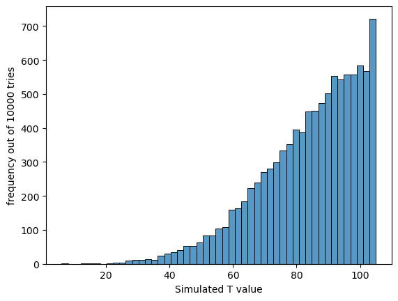
proportion of simulated datasets in which T<=46 = 0.0255

We obtain a value of $T$ as extreme as the one in our real dataset about 2.5% of the time.

The p value of the test, which is the same as the proportion of simulated datasets in which T<=46, is about 0.025 or 2.5% (it will vary slightly each time you run the code as the null distribubtion is built from random samples). This is not a bad match for the value we got from the built-in function, which was 0.0266 or 2.66%