10.7. Permutation testing - more practice

We will work with the (made up) wellbeing survey data that we used for the exercises on bootstrapping.

The aim of these exercises is to give you some practice running permutation tests and deciding what to permute and what your test statistic is in each case!

Set up Python libraries

As usual, run the code cell below to import the relevant Python libraries

# Set-up Python libraries - you need to run this but you don't need to change it
import numpy as np
import matplotlib.pyplot as plt
import scipy.stats as stats
import pandas 
import seaborn as sns

Import and view the data

wb = pandas.read_csv('https://raw.githubusercontent.com/jillxoreilly/StatsCourseBook/main/data/WellbeingSample.csv')
wb

	ID_code	College	Subject	Score_preVac	Score_postVac
0	247610	Lonsdale	PPE	60	35
1	448590	Lonsdale	PPE	43	44
2	491100	Lonsdale	engineering	79	69
3	316150	Lonsdale	PPE	55	61
4	251870	Lonsdale	engineering	62	65
...	...	...	...	...	...
296	440570	Beaufort	history	75	70
297	826030	Beaufort	maths	52	49
298	856260	Beaufort	Biology	83	84
299	947060	Beaufort	engineering	62	65
300	165780	Beaufort	PPE	48	56

301 rows × 5 columns

1. For engineering students, is wellbeing increased after the vacation compared to before?

We hypothesise that engineering students will feel better after the vacation. Test the hypothesis using a permutation test.

Let’s get just the rows of the dataframe containing engineering students:

wb[wb['Subject']=='engineering']
# OR - 
# wb.query('Subject == "engineering"')
# see Sammi's coding support sheet

	ID_code	College	Subject	Score_preVac	Score_postVac
2	491100	Lonsdale	engineering	79	69
4	251870	Lonsdale	engineering	62	65
6	841260	Lonsdale	engineering	71	58
7	960120	Lonsdale	engineering	54	54
15	670880	Lonsdale	engineering	70	69
...	...	...	...	...	...
266	842870	Beaufort	engineering	52	58
278	414020	Beaufort	engineering	76	82
291	384240	Beaufort	engineering	78	89
294	457900	Beaufort	engineering	72	62
299	947060	Beaufort	engineering	62	65

61 rows × 5 columns

Things you need to decide:

• what is our null hypothesis

• what is our alternative hypothesis?

Is it a paired or unpaired test?

• therefore which permutation_type is needed, samples, pairings or independent?

• are we testing for the mean difference (within pairs) mean(x-y), or the difference of means mean(x)-mean(y)

• what actually are x and y in this case?

Is it a one- or two-tailed test?

• therefore which alternative hypothesis type is needed, two-sided, greater or less?

What $\alpha$ value will you use?

• what value must $p$ be smaller than, to reject the null hypothesis?

• this is the experimenter’s choice but usually 0.05 is used (sometimes 0.001 or 0.001)

The answers to the things you need to decide!

$\mathcal{H_0}$: The mean difference in wellbeing post-pre vacation is zero for engineering students

$\mathcal{H_a}$: The mean difference in wellbeing post-pre vacation is greater than zero, ie wellbeing improves over the vacation.

This is a paired test as we are comparing each person’s wellbeing before the vacation to their own wellbeing after the vacation. Therefore we are testing the mean difference mean(x-y) and need to shuffle the samples (flip pre and post labels with pairs, but don’t break the pairings)

# define a funtion that gives the mean difference for two series x and y
def mDiff(x,y):
    return np.mean(x-y)

It’s a one-tailed test because our hypothesis is directional (we expect wellbeing to increase after the vacation) and if we calculate of difference as post-pre, a significant effect would be a big positive difference, so we need alternative='greater'

We will test at the 5% ($\alpha=0.05$) level

Run the test!

Here is some code to run the test

post = wb[wb['Subject']=='engineering']['Score_postVac']
pre = wb[wb['Subject']=='engineering']['Score_preVac']

stats.permutation_test((post,pre), mDiff, alternative='greater', permutation_type='samples', n_resamples=10000)

PermutationTestResult(statistic=1.0491803278688525, pvalue=0.22717728227177283, null_distribution=array([-1.21311475,  2.26229508, -0.16393443, ...,  2.55737705,
       -0.26229508,  0.39344262]))

Is it significant?

Reading the test output:

statistic=1.0491803278688525

The mean post-pre wellfare score difference in our ‘real’ sample was 1.049 points (welfare was 1.049 points higher after the vac - this is a small increase as it’s a 100-point scale)

pvalue=0.214

The probability of obtaining such a large increase in welfare due to chance if there was really no effect of the vacation is 21.4%

Conclusions

We fail to reject the null hypothesis as $p$ is not smaller than $\alpha$

How would you write that up in a journal article?

We hypothesised that wellbeing increased over the vacation. We compared wellbeing in engineering students (n=61) before and after the vacation using a paired samples permutation test. There was no significant increase in wellbeing after the vacation (mean difference is an increase of 1.049 points, p=0.214, one tailed).

2. Do does wellbeing (before the vacation) differ between history and maths students?

We hypothesise that students studying different subjects may have different levels of wellbeing but we don’t have an a priori expectation about which subjects will have higher wellbeing.

Test the hypothesis using a permutation test.

Let’s get just the prevacation wellbeing scores for history students an just maths students:

history = wb[wb['Subject']=='history']['Score_preVac']
maths = wb[wb['Subject']=='maths']['Score_preVac']

Things you need to decide:

• what is our null hypothesis

• what is our alternative hypothesis?

Is it a paired or unpaired test?

• therefore which permutation_type is needed, samples, pairings or independent?

• are we testing for the mean difference (within pairs) mean(x-y), or the difference of means mean(x)-mean(y)

• what actually are x and y in this case?

Is it a one- or two-tailed test?

• therefore which alternative hypothesis type is needed, two-sided, greater or less?

What $\alpha$ value will you use?

• what value must $p$ be smaller than, to reject the null hypothesis?

• this is the experimenter’s choice but usually 0.05 is used (sometimes 0.001 or 0.001)

The answers to the things you need to decide!

$\mathcal{H_0}$: The difference mean wellbeing pre vacation for history and maths students is zero

$\mathcal{H_a}$: The difference mean wellbeing pre vacation for history and maths students is non-zero, ie one subject has higher wellbbeing

This is an independent samples test as we are comparing each person’s wellbeing before the vacation to their own wellbeing after the vacation. Therefore we are testing the mean difference mean(x)-mean(y) and need permutation_type = 'independent' (shuffle which datapoints are labelled ‘history’ or ‘maths’ but keep the number of students labelled as history and maths matching the original sample)

# define a funtion that gives the mean difference for two series x and y
def dMeans(x,y):
    return np.mean(x)-np.mean(y)

It’s a two-tailed test because our hypothesis is non-directional (we don’t have particular predictions about which subject we might have higher wellbeing, we are just interested in whether there is a difference) so we need alternative=’two-sided’

We will test at the 5% ($𝛼=0.05$) level

Run the test!

Here is some code to run the test:

stats.permutation_test((history,maths), dMeans, alternative='two-sided', permutation_type='independent', n_resamples=10000)

PermutationTestResult(statistic=3.486388384755003, pvalue=0.17638236176382363, null_distribution=array([ 4.61887477,  2.00544465,  0.87295826, ...,  0.52450091,
       -0.43375681, -2.43738657]))

Is it significant?

Reading the test output:

statistic=3.486388384755003

The difference in mean welfare score in our ‘real’ sample was 3.49 points (welfare was 3.49 points higher for history students)

pvalue=0.16718328167183283

The probability of obtaining such a large difference in welfare due to chance if there was really no effect of the subject is 16.7%

Conclusions

We fail to reject the null hypothesis as $p$ is not smaller than $\alpha$

How would you write that up in a journal article?

We hypothesised that wellbeing might differ between students in different subjects. We compared wellbeing in maths students (n=29) and history students (n=19) before the vacation using an independent samples samples permutation test. There was no significant difference in wellbeing between subjects (difference of means = 3.48 points, p=0.167, two tailed).

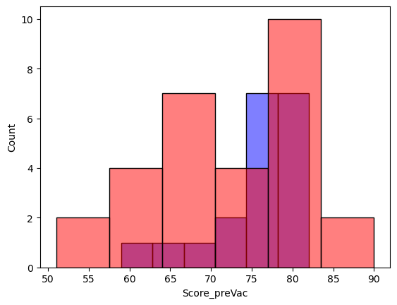
Out of interest, why was this large difference not significant?

Probably because tha variation in welfare within each group was relatively large, and the sample size was relatively small:

sns.histplot(history, color='b', alpha=0.5)
sns.histplot(maths, color='r', alpha=0.5)
plt.show()

3. Are welfare scores pre- and post-vac correlated for biology students?

We hypothesise that there is a strong individual difference effect on welfare scores and that scores pre- and post-vac are correlated. Let’s say the sample we have availablbe to test this are biology students.

Test the hypothesis using a permutation test.

Let’s get two series containing the data we need:

prevac = wb[wb['Subject']=='Biology']['Score_preVac']
postvac = wb[wb['Subject']=='Biology']['Score_postVac']

Plot the data

A scatterplot may help us get a sense of whether there is a correlation

sns.scatterplot(x=prevac, y=postvac)

<Axes: xlabel='Score_preVac', ylabel='Score_postVac'>

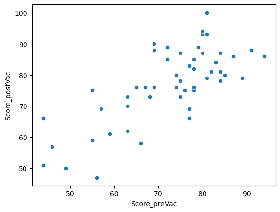
…looks like there is a correlation. Let’s test it.

The answers to the things you need to decide!

$\mathcal{H_0}$: The correlation in wellbeing pre- and post- vacation is zero for students in Lonsdale college

$\mathcal{H_a}$: The correlation in wellbeing pre- and post- vacation is greater than zero (students with high wellbeing bbefore the vac also have high wellbeing after the vac)

As this is a correlation, we need permutation_type = 'pairings' (shuffle which datapoints are paired with which)

# define a function that gives the correlation for two series x and y
# note that np.corrcoef returns a 2x2 matrix so we need to get just the relevant element
def mycorr(x,y):
    c = np.corrcoef(x,y)
    return c[0,1]

It’s a bit ambiguous whether a one- or two-tailed test is needed here.

The question does not state the expected direction of effect, which would suggest a two tailed test.

However, there is really only one reasonable direction in which a correlation could be expected, namely a positive correlation (we expect the students with the highest wellbeing before the vac also have highest wellbeing after the vac, hence we expect a positive correlation coefficient) - the reverse (students with high wellbeing before the vac have low wellbeing after) is nonsensical. So on the basis of common sense you could argue for a one-tailed test (and hence use alternative='greater).

Either of these is an acceptable answer as long as you briefly explain your decision.

We will test at the 5% ($𝛼=0.05$) level

Run the test!

Here is some code to run the test:

stats.permutation_test((prevac,postvac), mycorr, alternative='greater', permutation_type='pairings', n_resamples=10000)

PermutationTestResult(statistic=0.7401813753937694, pvalue=9.999000099990002e-05, null_distribution=array([ 0.16350452, -0.23928463,  0.14995842, ...,  0.18976737,
        0.02292917, -0.02365283]))

Is it significant?

Reading the test output:

statistic=0.7401813753937694

The correlation between pre and post vac wellbeing scores in out ‘real’ sample was 0.74

pvalue=9.999000099990002e-05

The probability of obtaining such a large difference in welfare due to chance if there was really no effect of the subject is 9.99 x $10^{-5}$%, which is 0.0000999 or about one in ten thousand

Conclusions

We reject the null hypothesis as $p$ is much smaller than $\alpha$ and conclude there is a correlation between wellbeing scores pre and post vacation

How would you write that up in a journal article?

We hypothesised that wellbeing before and after the vacation would be correlated across individuals. We calculated Pearson’s $r$ for a group of biology students (n=51) before and after the vacation, and tested its significance using a permutation test. There was a highly significant positive correlation (r=0.74, p<0.0001, one tailed), meaning that students with higher wellbeing before the vacation also had high wellbeing after the vacation.