1.3. Using Anaconda and JupyterLab

For instructions on working in Colab, see the next section of these notes

In this section you will see how to:

• Access ready-made example Jupyter Notebooks in JupyterLab

• Create your own Jupyter Notebbooks

• Download and read data files including those downloaded from Canvas

Read through and check you can complete the Exercise at the bottom of this page

1.3.1. Anaconda

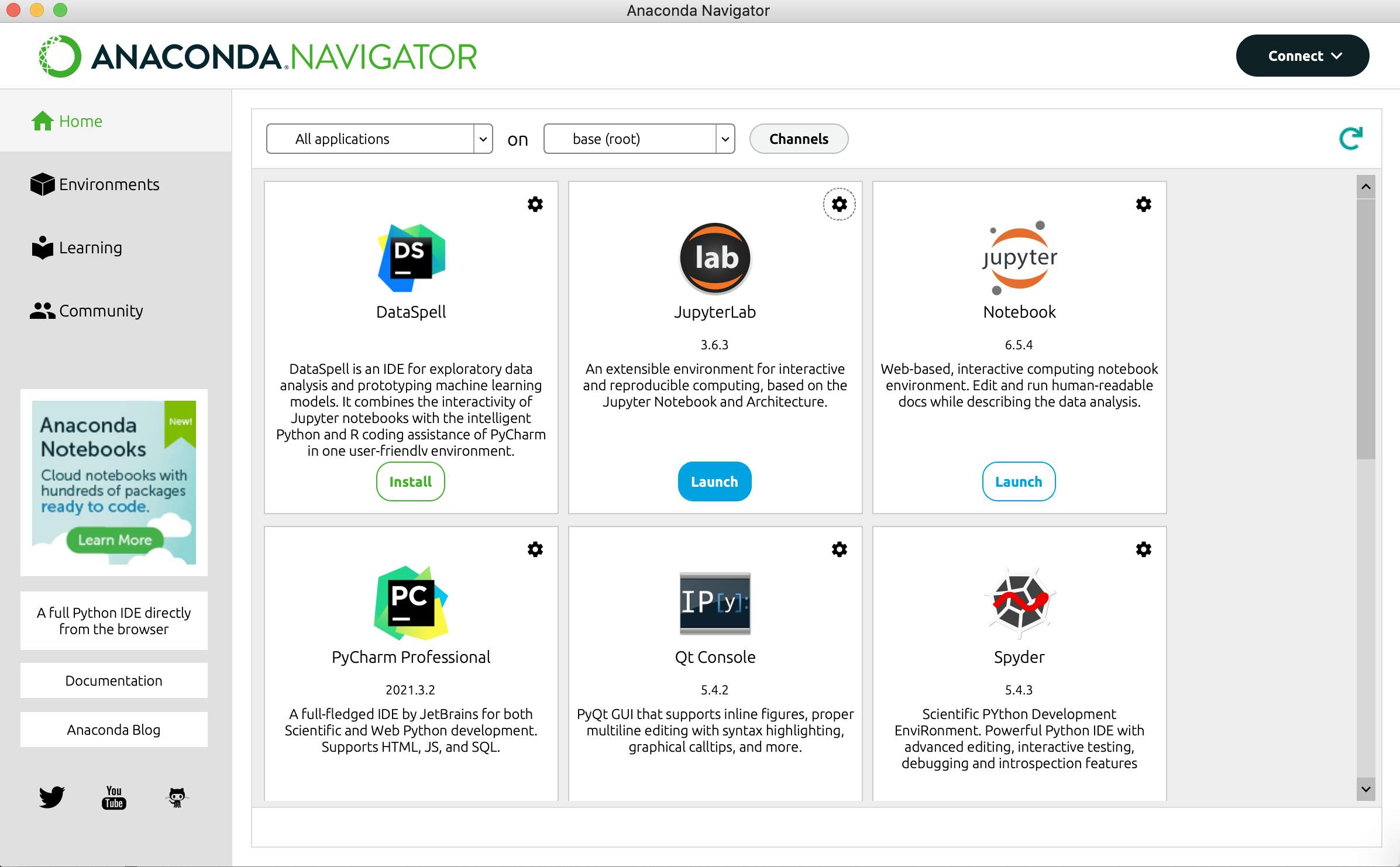
Once you have installed Anaconda Navigator on your computer, you will be able to open it from the Start Menu or Finder. It should be near the top of the list of Applications (because Anaconda begins with A!) and has a green circle symbol (actually an Ouruboros).

When you open Anaconda Navigator, you will see a window with lots of tiles for different Python-related apps:

1.3.2. JupyterLab

We will be using JupyterLab to work with Jupyter Notebooks. You can Launch JupyterLab from Anaconda Navigator by clicking “Launch”.

JupyterLab will open, not as its own window, but as a tab in your default Web Browser

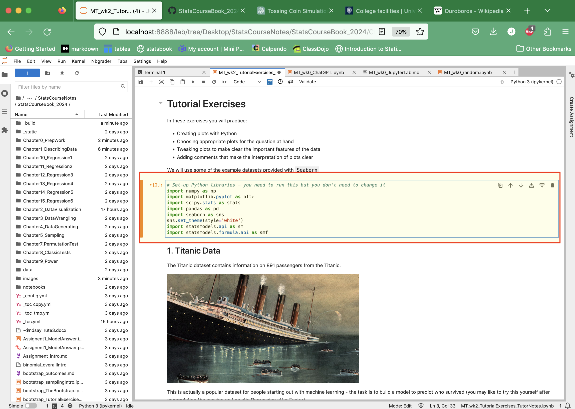
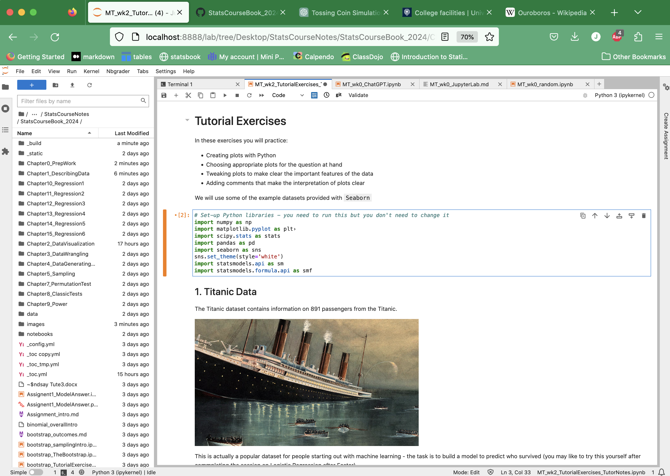
File navigator

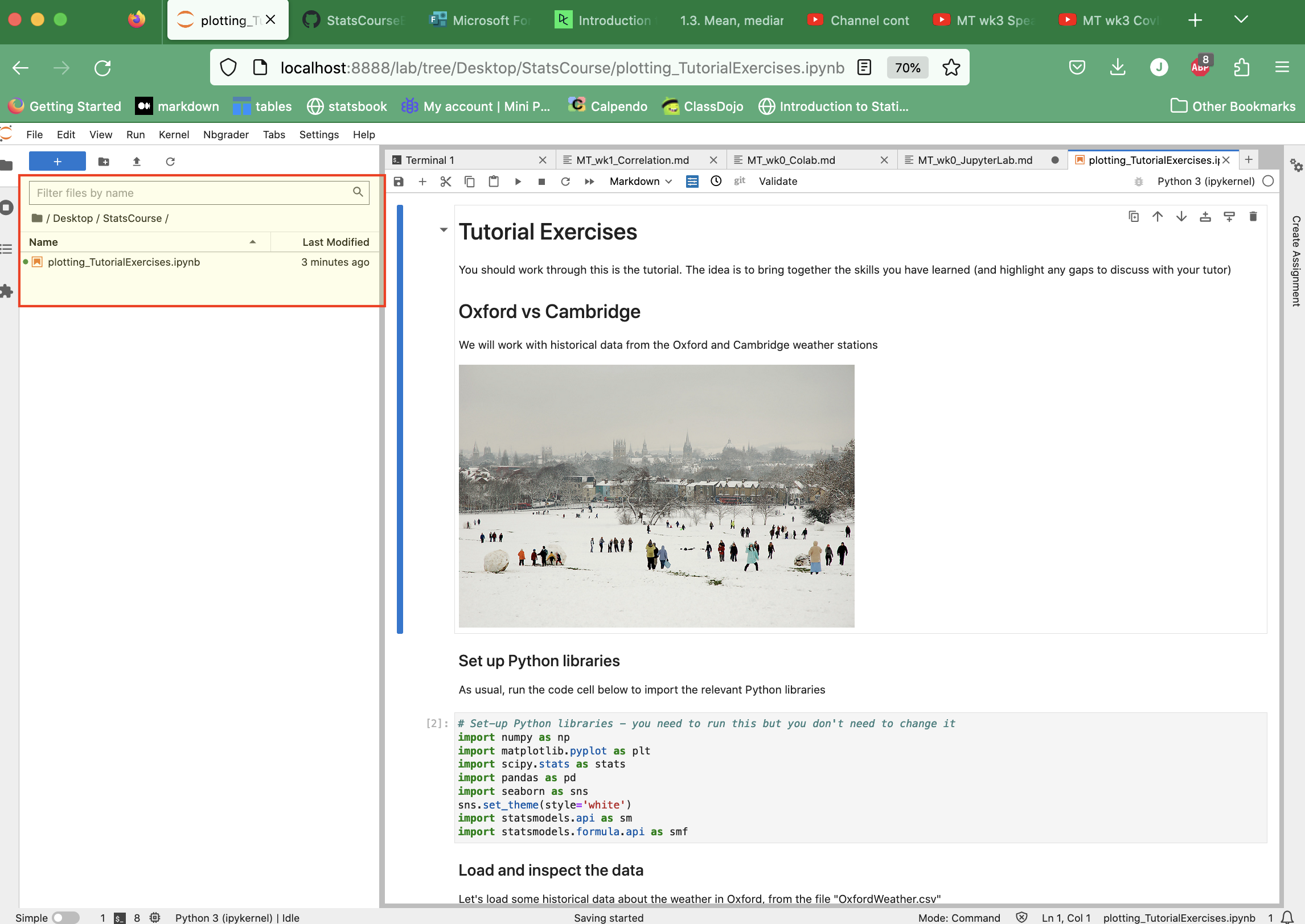
At the left of the window you will see a file navigator - this shows you the files in your current folder.

It is a good idea to create a folder (eg on your Desktop) to keep the documents for this course. Say for example you create a folder on your desktop called “StatsCourse”. You can navigate to this folder using the browser pane in JupyterLab and can the open documents (such as the downloaded Jupyter Notebook) by double clicking them.

Workspace

On the right there is a window where the Jupyter Notebooks themselves are opened.

1.3.3. Exercise 1: Open an existing Notebook

First we will explore the Jupyter Notebook format using a ready made notebook downloaded from the course notes website.

These course notes are made up of some pages that are just text (“Markdown”) and some that are actual Jupyter Notebooks.

Any file that is an actual Jupyter Notebook can be downloaded automatically to your computer by clicking the download button and selecting .ipynb, which is the extension for Jupyter Notebook files

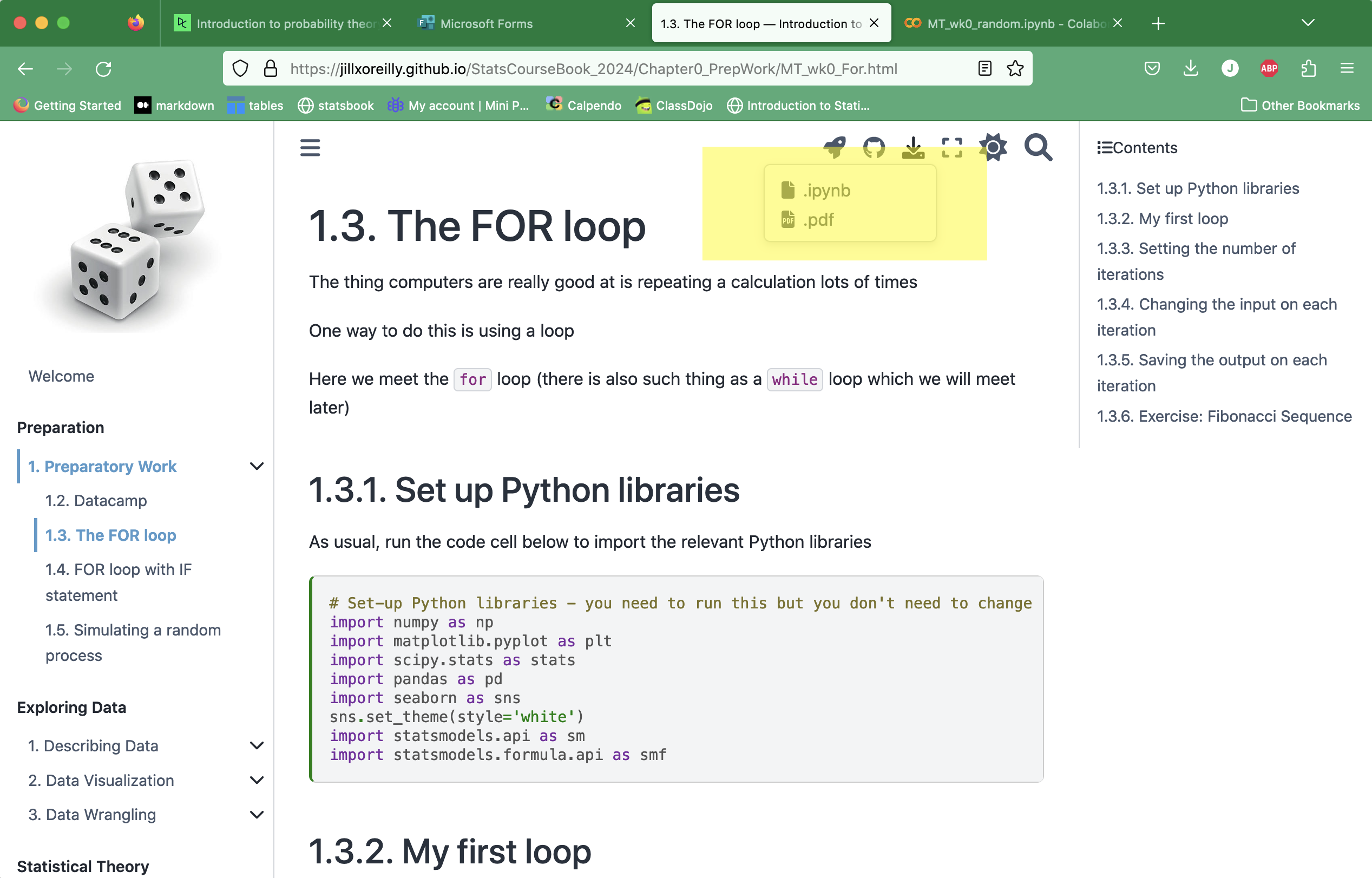
• The file will go to wherever internet downloads go on your computer - probably your Downloads folder!

• Move it to the folder you have created for this course

• Open it in JupyterLab by going to JupyterLab, finding the file in the file browser pane at the left of the screen, and double-clicking it.

You can now run and/or edit this Notebook file!

Markdown cells

Cells with text and images are called Markdown cells. Markdown refers to the codes we use to format the text in these cells, for example headings are indicated by hashtags (one hash is the biggest heading, more hashes = smaller subheadings)

If you double-click a markdown cell, you can edit the text, and can also see these markdown symbols.

For your purposes, probably the only ones you need to know are:

• Bullet points are indicated by * at the start of the line

• Titles are indicated by hashtags

• Bold font is indicated by double-star **text** –> text

• Italic font is indicated by single-star *text* –> text

You can find examples of all of these in my example notebooks

Code cells

These contain Python code

Note that any code preceded by a hashtag # is a comment - explanatory text that is visible to human readers but is ignored by the computer

• Sometimes I comment out code in notebooks that I don’t want to automatically run - you can then uncomment it (by removing the hashtags at the start of the lines) when you are ready to run it.

• The code block below is “commented out” - students are invited to think ahead about what the output of the code will be, before deleting the hashtags and running the code to check their answer.

You can choose the cell type (you will want either Code or Markdown) from a dropdown box.

• If you forget to do this it will default to code which will probably then give you an error message if you write something in the cell that is not code

• If this happens, simply change the cell type via the dropdown box.

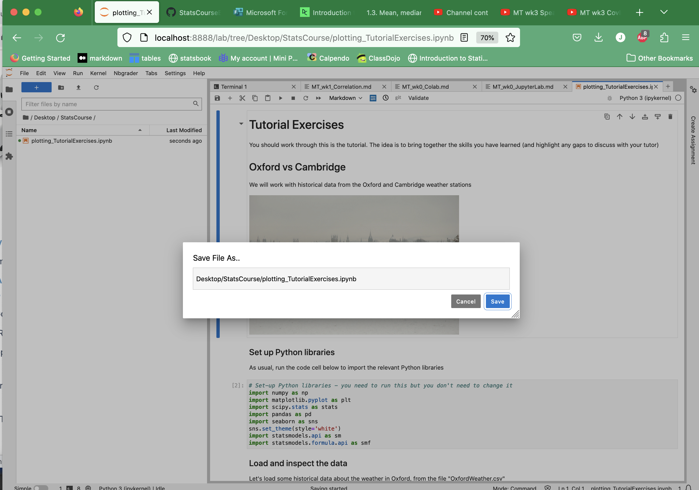
Saving your work

Don’t forget to save your work! You can do this via the File menu in the top left of the JupyterLab Window.

Click File –> Save Notebook As

A dialogue box appears where you should enter the filename, including the complete path (folder your file is going into). Check that this path is correct - it will be automatically filled in to save the file in the folder you are “in” in the file browser pane (at the left of the screen).

1.3.4. Exercise 2: Creating a New Notebook

Now let’s try to create a totally new notebook. You will see there are a couple of things we have to do to ‘set up’ the notebook.

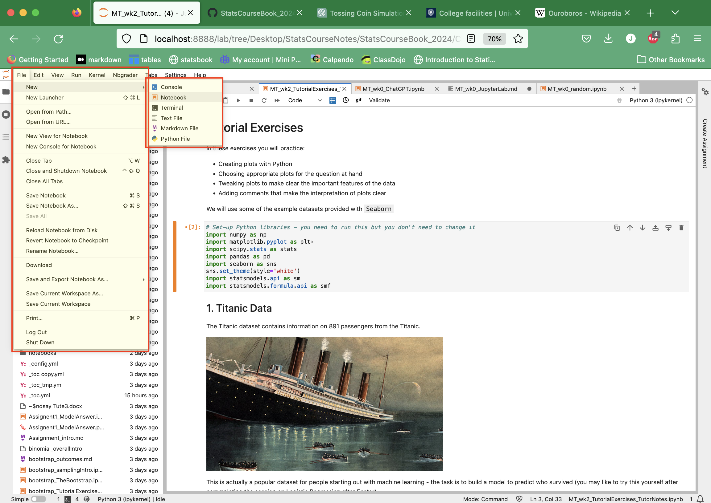
Create a new Notebook file

You can create a new Jupyter Notebook by clicking File –> New –> Notebook:

Import Python libraries

At the top of each Notebook you will need to import the Python libraries that are used in the Notebook

You will see the same block of code repeated in all my example notebooks; this imports the libraries we use in this course

You will need to copy this block into any new notebooks you create

• You could add other libraries to the input list if you found one you wanted to use (another plotting library for example)

1.3.5. Exercise 3: Load data

This is a statistics course, so of course we will need to work with data files!

You may be used to seeing data in files such as Excel spreadsheets. Often data are stored in text files such as .csv (comma separated values) files. This is a generic file type that can be read by Excel, Numbers, and by programming tools such as Python, R and Matlab.

We will generally be reading .csv data files into Python as Pandas dataframes. This can be done using the tool pd.read_csv() as in the exercise below.

• From Canvas, downlad the example data file ‘ExampleData.csv’

  • Save it in the folder you made for this course, eg Desktop/StatsData

• In your Jupyter Notebbook, use the following code to load the data as a Pandas dataframe:

cats = pd.read_csv('ExampleData.csv')
display(cats)

• You may prefer to create a folder inside IntroSession called data and put the ExampleData.csv in there

  • If so use the following code to load it:

data = pd.read_csv('data/ExampleData.csv')
display(cats)

What is in the data file?

The example data file is a text file (.csv) with words (column headers) and numbers in it.

This is a universal file type for storing data and can be opened by other programmes such as Excel

• If you like, you can open ExampleData.csv in a text editor (such as TextEdit) to have a look at it

Once we read it into Pandas it is in the computer’s memory so to speak, in a formmat that Python recognizes and upon which we can perform statistical operations (like testing for a difference between the values in two columnms of the datafiles).

Note - loading data in example notebooks

In the example notebooks on this course notes website, I tend to pull the data directly from my GitHub (a web-based platform where the course files are stored). This just means that you can run the examples without having to separately download data files and edit the code etc.

For files pulled from GitHub, the filename will be a URL (web address) rather than a filename in a folder on your computer. You don’t need to know how to fill in these URLs, I’m just explaining why these look different to the Data Loading example below.