1.5. Skew#
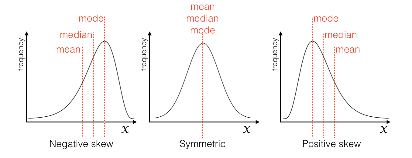
Data distributions are said to be skewed when there is a long tail of values to one side of the peak:

When a distribution is symmetrical (no skew), the mean, median and mode tend to coincide (fall on top of each other).
However, when a distribution has positive skew (a long tail of high values) the mean is dragged up above the median, and conversely when a distribution has negative skew (a long tail of low values) the mean is dragged down below the median.
To work out whether a dataset is skewed or symmetrical, we would need to plot the data (usually in a histogram). More on plotting in the next chapter.
1.5.1. Boundaries can cause skew#
Skew often arises in cases where there is a natural boundary to the range of possible data values.
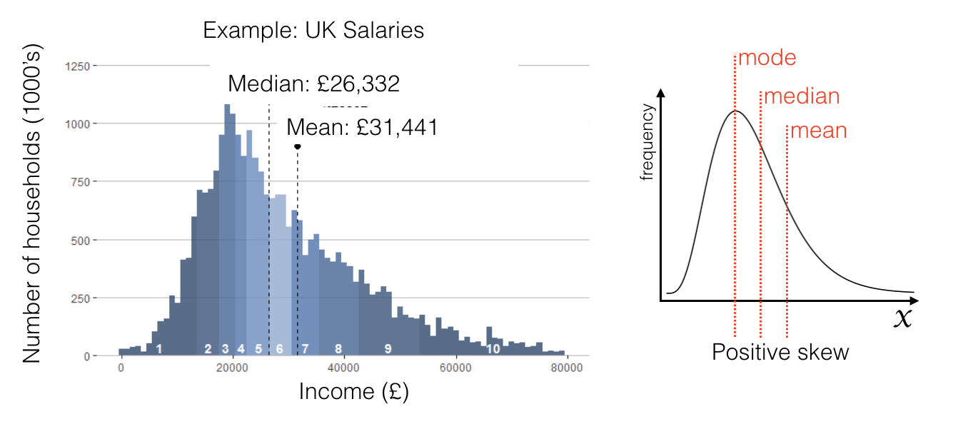
For example, the distribution of income is highy positively skewed.

The median income is around £26,000.
Nobody’s income can be more than £26,000 below the median income (as you can’t earn less than £0)
However some people do earn much more than £26,000 creating a long tail of high incomes
Similarly, the distribution of age at death in modern times is negatively skewed.

the median age at death in the UK is 78
a lifespan could be 78 years shorter than the median (if someone sadly died as a baby)
a lifespan cannot be 78 years longer then the median as this would mean the person was 156 years old
Video#
Here is a video of me talking about skew and its interpretation.
