
2.5. Bayes Theorem#
Bayes theorem is stated as follows:
If we know the conditional probability \(p(B|A)\) and the two marginals \(p(A)\) and \(p(B)\), we can work out the final element \(p(A|B)\).
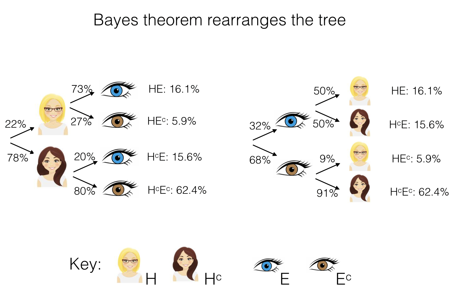
In other words, Bayes theorem allows us to reverse the structure of our probability tree - say we know the probabilities associated with the branching structure on the left - Bayes lets us work out the probabilities associated withthe branching structure the right (note these are not the same as each other!):
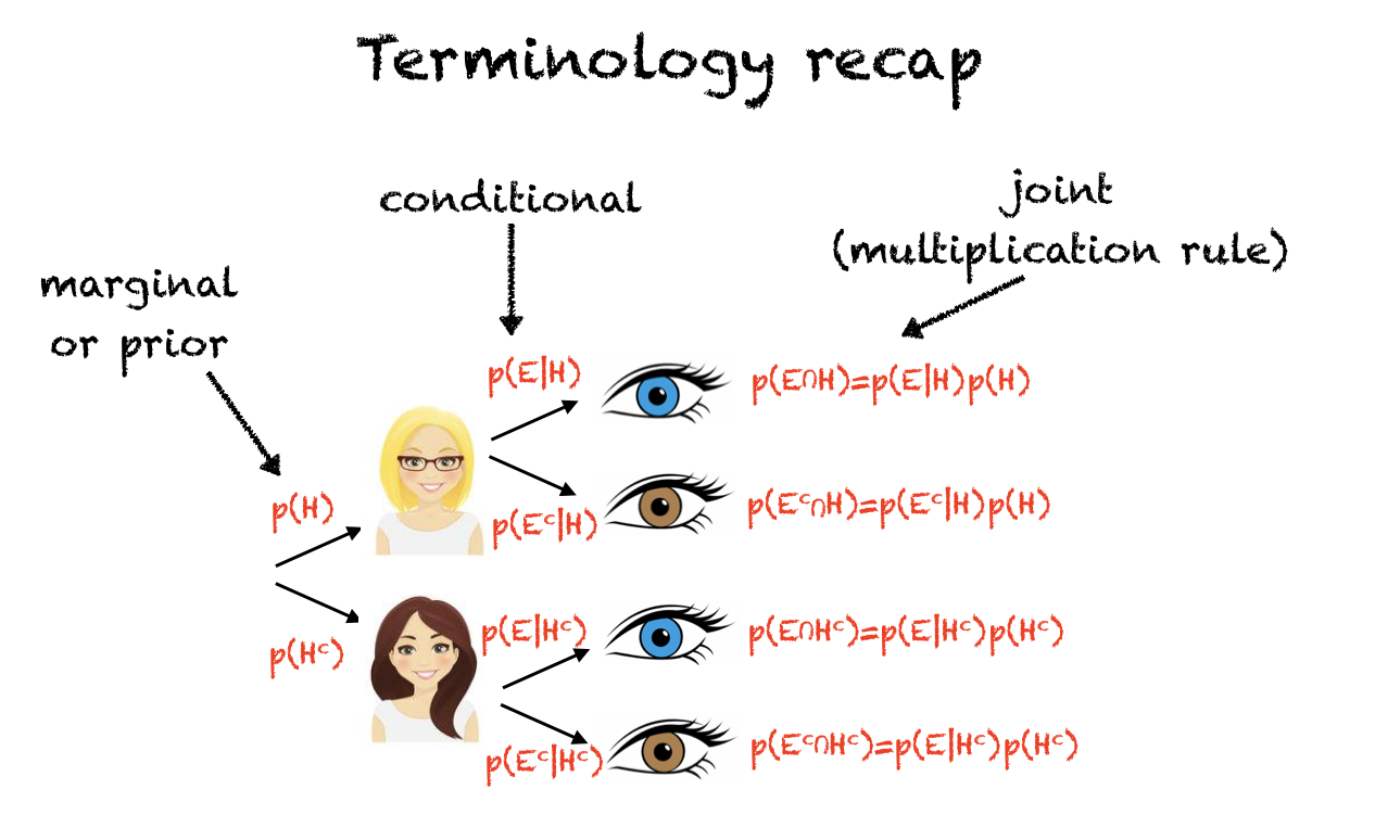
Here’s a recap of what all the different probabilities on the tree are in terms of probability notation:
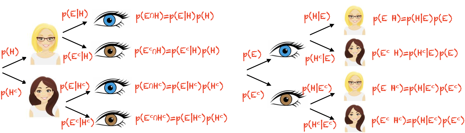
And here we can see that the roles of H and E are reversed when we reverse the order of the tree:
2.5.1. Inferring cause from data#
You may well be thinking, why is this so important?
Well, Bayes was interested in probability trees where not all the probabilities could be observed simply by counting (you could solve the problem above by just counting how many people had each combination of hair and eye colour and putting them into a contingency table).
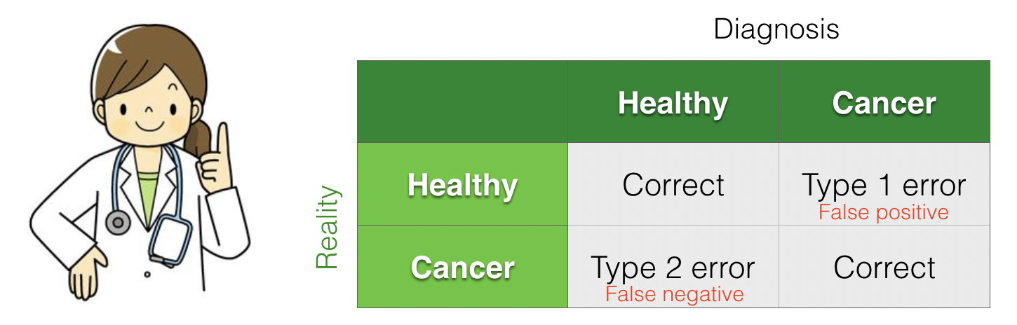
A key example of a probability tree where we can’t observe everying directly is in medical screening. We are able to observe the outcome of a screening test (such as a mammogram or ultrasound) and from this we must infer whether the patient has a disease (there is a true state of reality - disease or no disease - but this cannot be directly observed).
Because screens can be a true positive, correct reject, false positive, or false alarm, a positive screen doesn’t necessarily mean that the person has the disease.
Bayes Theorem allows us to interpret the results of a screening test correctly
Cancer screening example#
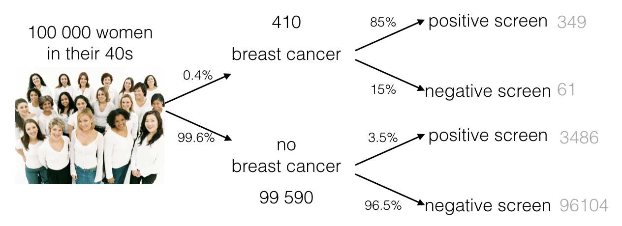
For example, say 100,000 women in their 40’s get routine screening for breast cancer:
Let \(C\) be the event that a woman has breast cancer
Let \(P\) be the event that a woman has a positive screening test result
Of course, we are interested in \(C\), but we can only observe \(P\)
Here is a probability tree (numbers based on true probabilities for this age group):
We could say a few things about the screening test itself, based on the conditional probabilities (the second branching point of the tree):
The sensitivity (power) of the test is 85%, because if a woman has breast cancer, there is an 85% chance of getting a positive screen
\(p(P|C)=0.85\)
The specificity of the test is 96.5%, because if a woman does not have breast cancer, there is only a 3.5% chance of getting a positive screen
\(p(P|C^c)=0.035\)
However, neither of these on their own tells the patient and their doctor what they need to know, which is not \(p(P|C)\) but rather, \(p(C|P)\).
Bayes theorem: p(cause|data)#
Out of the 100000 women, 3835 have a positive screen (alert for possible breast cancer). As one of those women, the patient needs to know what the probability is that she actually has breast cancer.
We can obtain this probability using Bayes theorem:
The marginal probabilty p(C) is found at the first branch point on the tree (0.4% of women in their 40s develop brest cancer, \(p(C)=0.004\)). This is sometimes called the prior probability of cancer (the probability we would say any woman had, before we had the information from the screening test).
The marginal probability \(p(P)\) is found by counting how many positive tests we have altogether from the 100000 women (349+3486 = 3835), so \(p(P) = 3835/100000 = 0.03835\)
Putting it all together we find that the probability a woman in her 40s has cancer, given the positive mammogram, is 0.088 (less than 10%).

That was surprising, wasn’t it?
Taking into account the prior probability was really important for interpreting the screening data. In fact breast cancer is rare in women in their 40s (sadly much more common in older age groups).
Because of the very high rate of false alarms (and related invasive medical procedures), routine screening is not offered to women below 50 on the NHS.
A similar principle applies to many medical screening problems. For example,
In antenatal screening for chromasomal disorders, evidence from ultrasound measurements and hormone levels is combined with a prior probability (which depends heavily on maternal age) to calculate a probability that the foetus has a chromasomal disorder.
During the coronavirus pandemic, the correct interpretation of a positive covid test (does the subject have covid?) varied enormously as the infection rate in the population rose and fell.
More informally, the most likely interpretation of symptoms (such as chest pain - heart attack or indigestion?) will depend on the prior probability of each cause in the patient’s demographic group.
Setting the cutoff#
We have previously seen that when setting a cutoff (the alpha value for a statistical test, or the clinically significant level of some measurement in a diagnostic test) we need to balance the probability of false positives and false negatives, and their implications.
We see now that the prior probability of each ground trust state of realiyy (the healthy and disease state, for example) is a further ingredient in this decision, as it also affects the probability of false positives and negatives.
