1.6. Correlation

Correlation, and the related measure covariance, tell us whether there is a relationship between two variables.

Consider the following (made up) dataset, containing scores of 100 children on English and Maths tests:

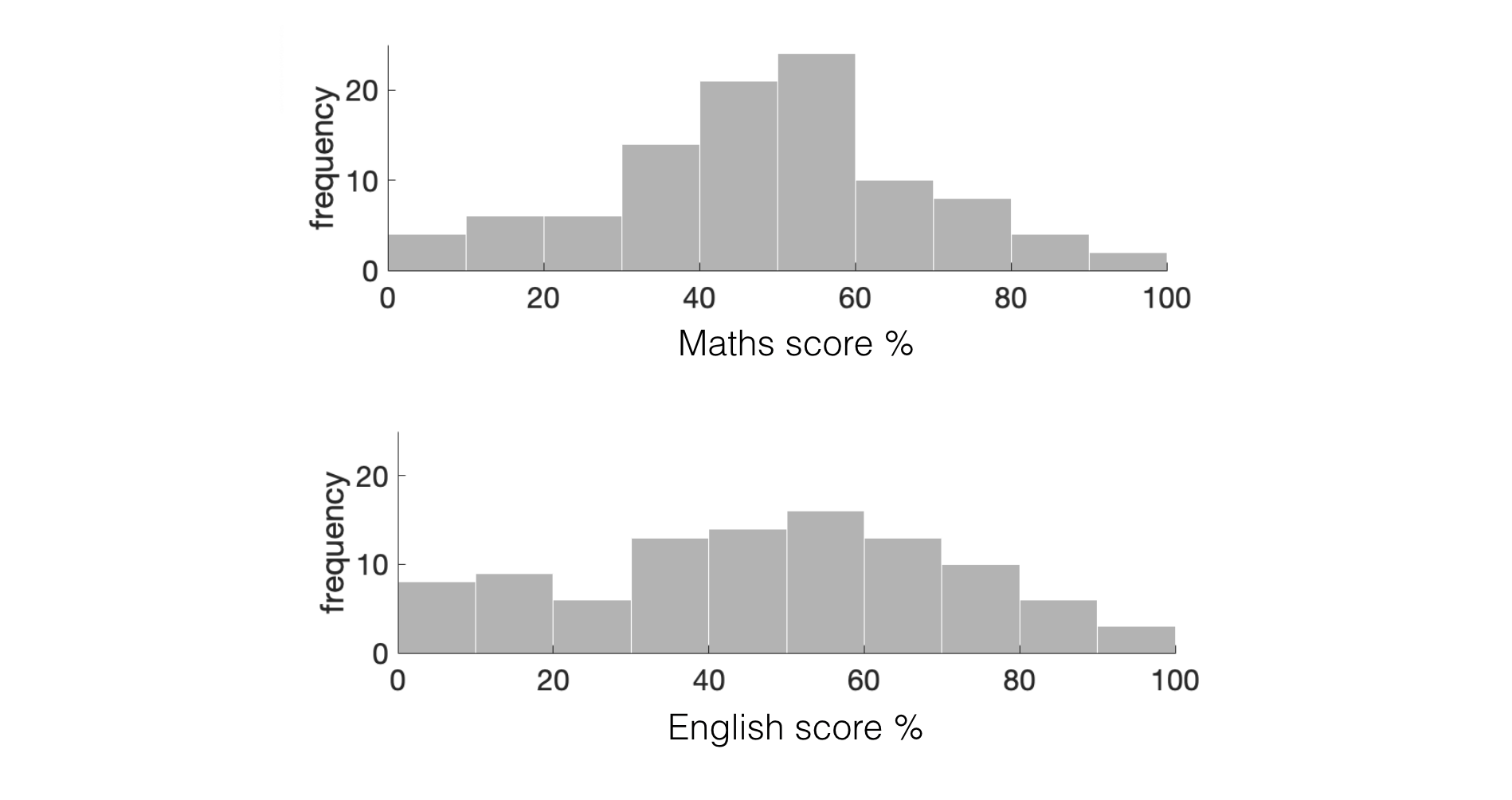
The histograms how us the distribution of scores on each test, but perhaps we are interested in a question we cannot answer from those histograms: do students who do well on the English test also do well on the maths test? This is a question about correlation.

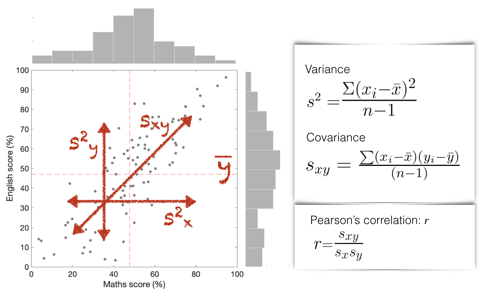
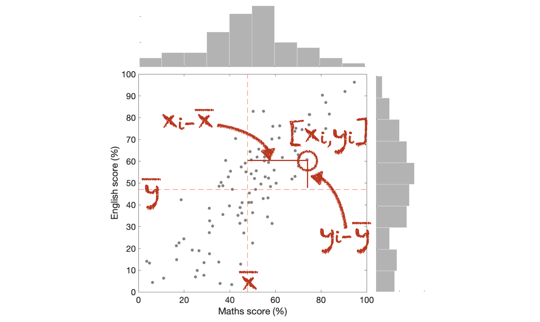
Here we present the data in a scatter plot which shows the relationship between the two variables: English score and Maths score. I’ve also replicated the histograms for each test in the margins.

Correlation and covariance are high when:

• There is a relationship between \(x\) and \(y\) (so knowing a student’s score on the maths test would really change our prediction of how well they did on the English test, or vice versa)

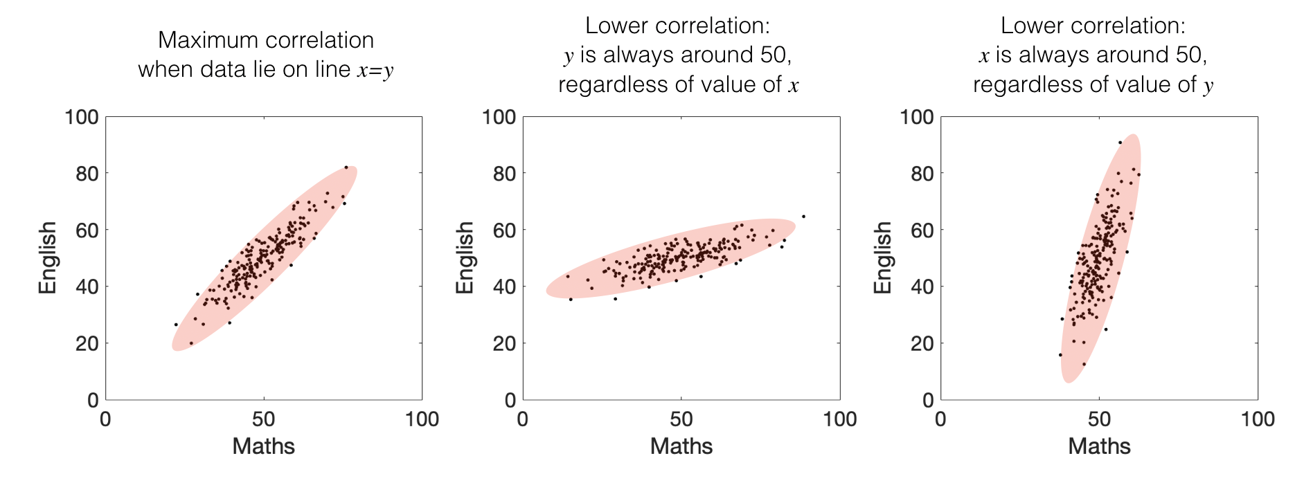
• When that relationship is tight (so most students did well on both tests or poorly on both, not well one one test and poorly on the other)

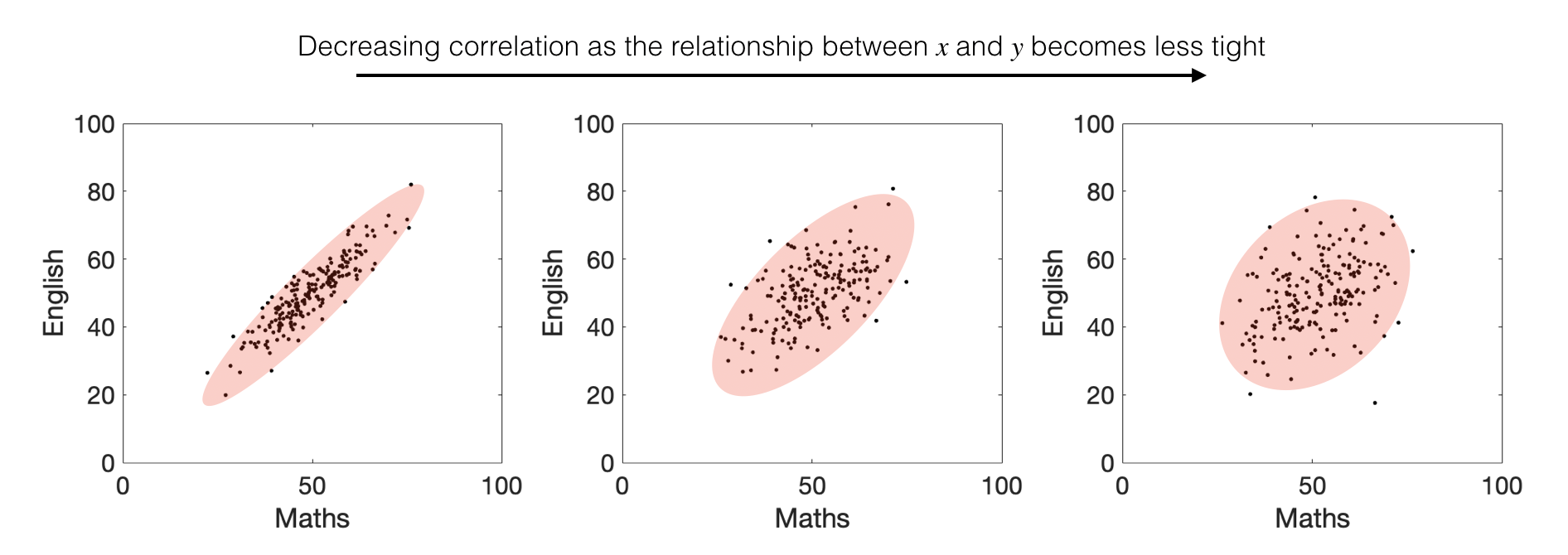
The correlation coefficient \(r\) is always a number between 1 (perfect positive correlation; all points on a line) and -1 (perfect negative correlation)

Correlation and covariance are closely related. As a descriptive statistic, correlation is most often used, as it gives us a ‘pure’ measure of the strength of the relationship between \(x\) and \(y\) (corrected for the spread within \(x\) and \(y\) independently).

1.6.1. Covariance

The variance in each variable, \(x\) (Maths score) and \(y\) (English score) is simply the standard deviation, squared.

This tells us how spread out the data points are for Maths and English - we can see from the histograms above that the data are slightly more spread out for Maths than English (the histogram for Maths is flatter).

A more mathematical way of thinking about variance (and standard deviation) is that they measure how far each data point is from the mean of the distribution:

Variance in \(x\), \(s^2_x\):

\[ s_x^2 = \sum\frac{(x_i - \bar{x})^2}{(n-1)} \]

Variance in \(y\), \(s^2_y\):

\[ s_y^2 = \sum\frac{(y_i - \bar{y})^2}{(n-1)} \]

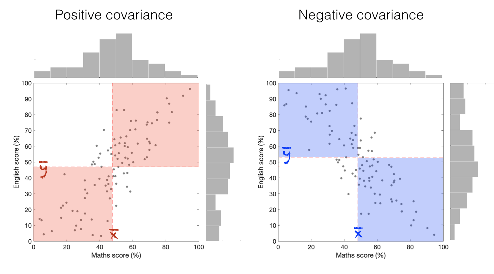
The covariance, in contrast, tells us whether the data are:

a. spread out such that high values in \(x\) tend to have high values in \(y\) (positive covariance)

b. spread out such that high values in \(x\) tend to have low values in \(y\) (negative covariance)

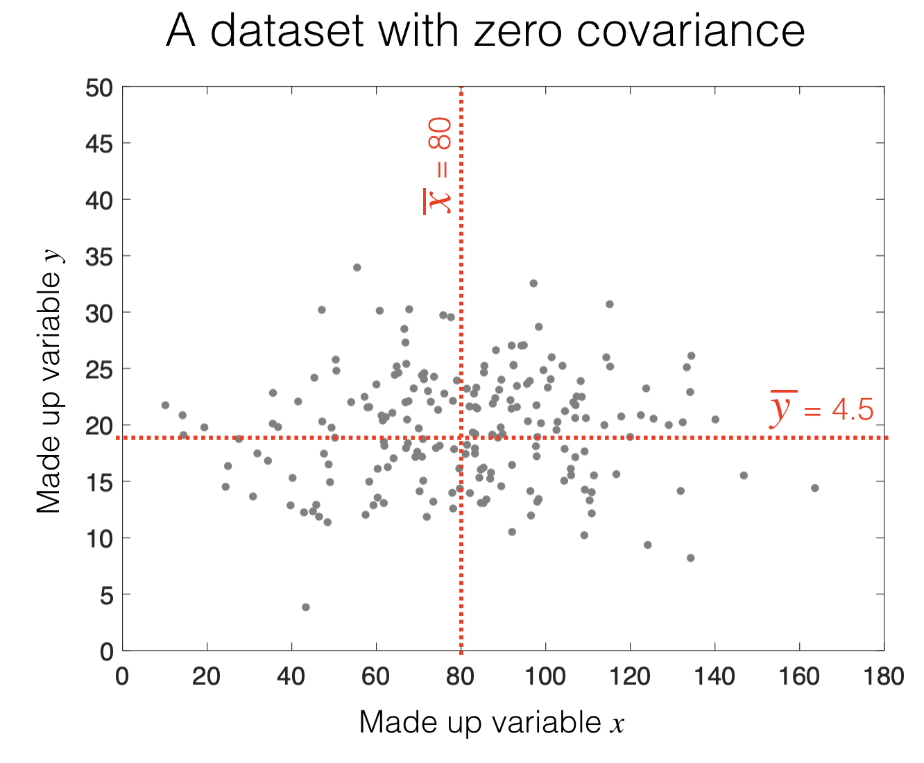
c. spread out such that high values in \(x\) are equally likely to have high or low values in \(y\) (no covariance)

We can see how this arises from the equation for covariance, \(s_{xy}\):

\[ s_xy = \sum\frac{(x_i - \bar{x})(y_i - \bar{y})}{(n-1)} \]

Each datapoint makes a contribution to the sum which can be positive (if \(x\) and \(y\) are both above the mean, or both below the mean) or negative (\(x\) is above the mean but \(y\) is below the mean, or vice versa).

The covariance is calculated by adding up these contributions for all data points:

• If most data points make positive contributions, covariance is large and positive

• If most data points make negative contributions, covariance is large and negative

• If there is an equal mixture of positive and negative contributions, covariance is small (near zero)

Here is a video of me explaining covariance:

1.6.2. Pearson’s Correlation \(r\)

Correlation is closely related to covariance, but is corrected for the spread in \(x\) and \(y\).

The most commonly used form of correlation, Pearson’s \(r\), is the covariance \(s_{xy}\), divided by the standard deviations in \(x\) and \(y\) (\(s_x\) and \(s_y\)):

\[ r = \frac{s_{xy}}{s_x s_y} \]

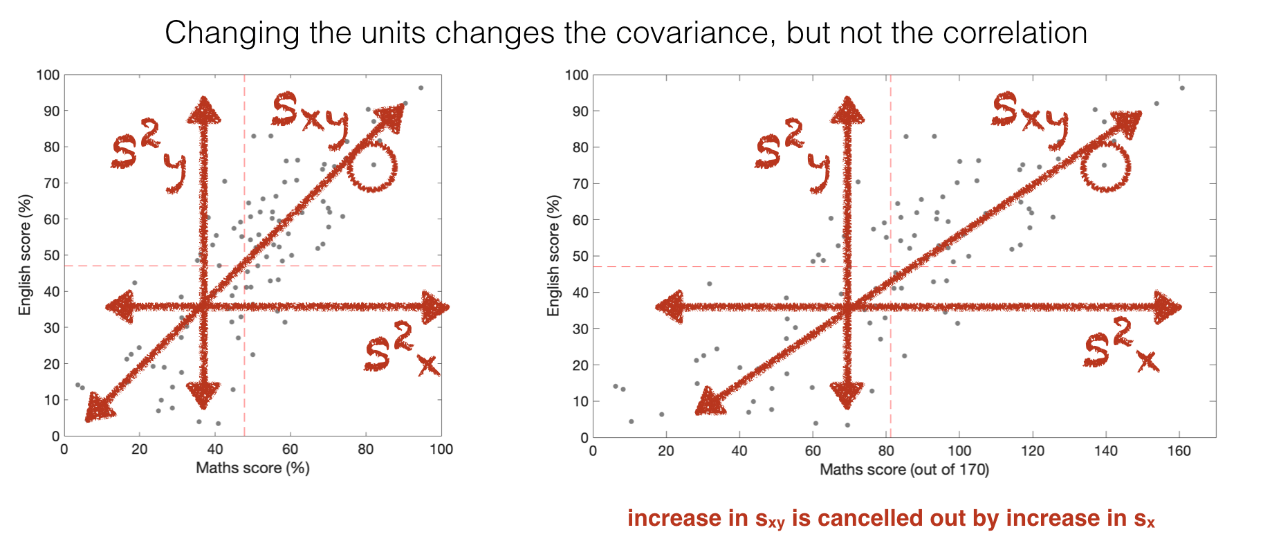
The effect of this is that correlation coefficient is not affected by linear transformations of \(x\) or \(y\) that change the variance in \(x\) or \(y\).

• linear transformations include adding a constant and multiplying by a constant

  • an everyday example would be changing the units - for example to get from temperature in \(^{\circ}C\) to temperature in \(^{\circ}F\), we multiply by \(9/5\) (multiplying by a constant) and add 32 (adding a constant).

  • The resulting values in F will be more spread out than the corresponding values in C - for example \(16^{\circ}C\) is \(61^{\circ}F\) and \(28^{\circ}C\) is \(82^{\circ}F\) - the difference is \(12^{\circ}C\) but \(21^{\circ}F\)

In our test scores example, imagine that maths scores were actually out of 170 points, but were converted to a percentage.

remember,

\[ r = \frac{s_{xy}}{s_x s_y} \]

• The covariance with English scores would be different depending on whether we use the raw Maths scores (out of 170) or the Maths scores expressed as percentages (so out of 100).

• The correlation is unaffected by this conversion, which makes it a ‘pure’ measure of the strength of assocation between \(x\) and \(y\).

Here is a video of me explaining the relationship between covariance and correlation:

Assumptions

Pearson’s correlation coefficient makes a number of assumptions:

1. The relationship between \(x\) and \(y\) is a straight line (not a curve)

2. That the variance in \(x\) and \(y\) is the same all along that line (no heteroscedasticity)

3. No bad outliers

These assumptions are illustrated below

If these assumptions are not met, it is preferable to use Spearman’s correlation coefficient instead.

1.6.3. Spearman’s Correlation \(r_s\)

In Spearman’s correlation, we replace the actual datapoints with their ranks, so the smallest data point becomes rank 1, the next smallest rank 2, etc. We then calculate Pearson’s correlation on the ranks, rather than the actual data.

Spearman’s \(r\) is equivalent to Pearson’s \(r\) for the ranks rather than the data values

When running correlations on the computer, we can simply set the argument method=spearman and the ranking etc is all done for us.

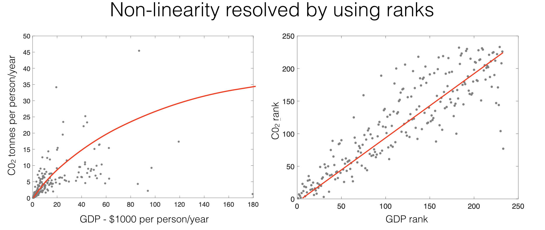
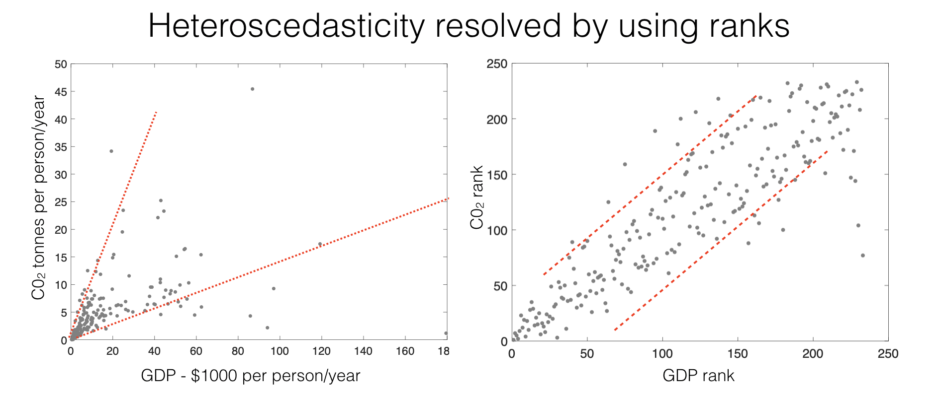
This solves the problems of linearity and heteroscedasticity, as seen in the CO2/GDP example:

• Whilst the relationship between GDP and CO_2 is curved, the relationship between ranks is linear

• Whilst the raw data show heteroscedasticity, the ranks do not

• The effect of outliers is minimzed by using ranks - the largest rank in the dataset \(x_1, x_2.... x_n\) is simply \(n\), whether the corresponding data value is 100 or 1000000.

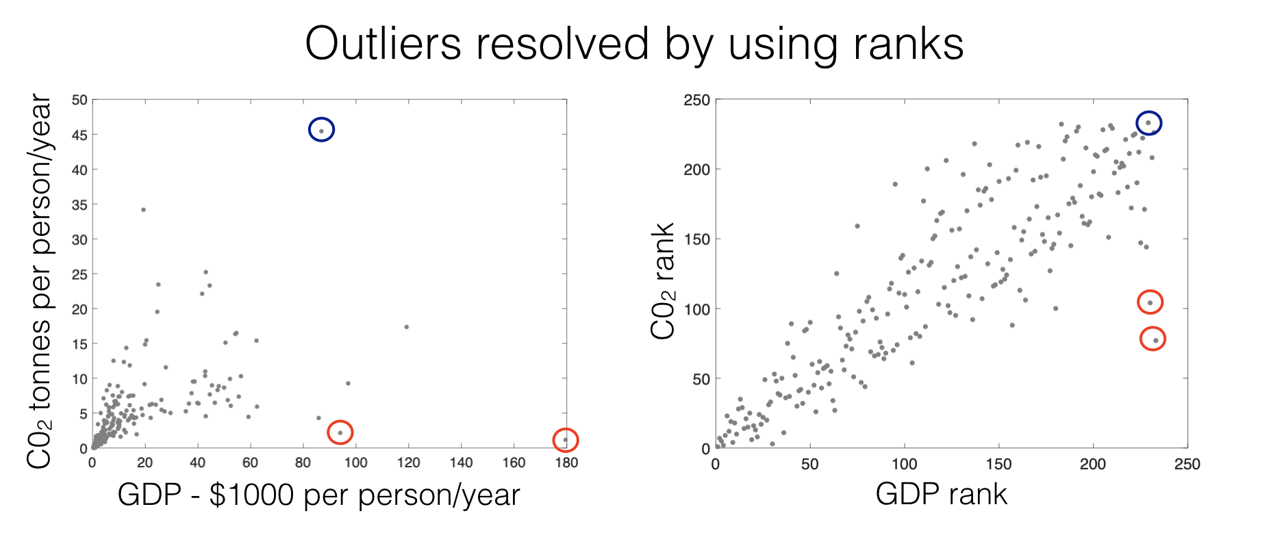
The marked data points are the same points in each plot - note how they move closer to the crowd in the ranked plot.

As with all rank-based statistics (see also: median, IQR and tests based on ranks such as the Rank-Sum Test), Spearman’s correlation requires few assumptions and is robust to outliers, but at the cost of ‘wasting’ some information (i.e. the exact numerical values of \(x\) and \(y\)). This idea will be explored further later in the course.

Video

Here is a video of me explaining the assumptions of Pearson’s correlation and why Spearman’s correlation coefficient helps when the assummptinos are violated.

• In the video I also show a formula for calculating Spearman’s from ranks - you don’t need to worry about this, it is sufficent to know how to change the correlation method in Python, and that Spearman’s \(r\) is equivalent to Pearson’s \(r\) for ranks.