3.3. Normal Distribution

The t-test is a test for difference of means that can be used if the data to be tested are drawn from a normal distribution.

Here we take a look at the normal distribution itself

3.3.1. Characteristics of the normal distritbution

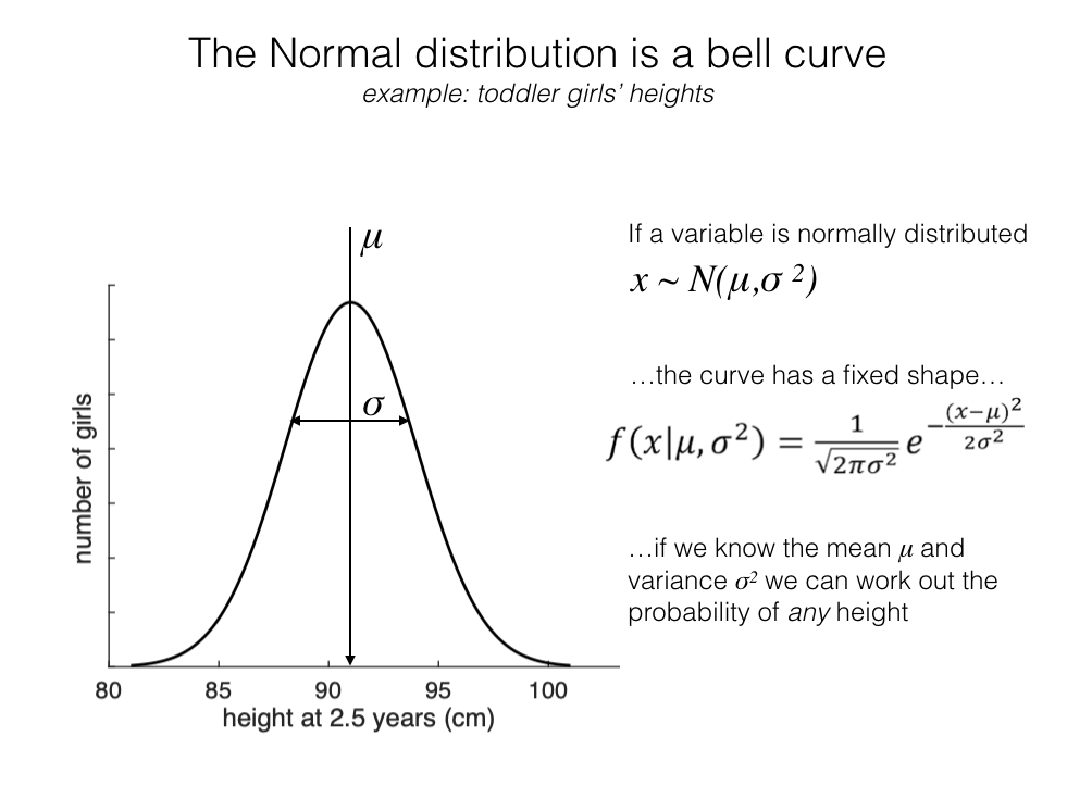
The normal distribution is a data distribution with a very particular ‘bell curve’ shape. It is not just any old symmetrical, unimodal distribution - it is described by an exact equation.

As we will later see that even the \(t\) distribution, which looks pretty similar, can be distinguished from the normal distribution, and this distinction is important in statistical testing.

Normal distribution has two parameters

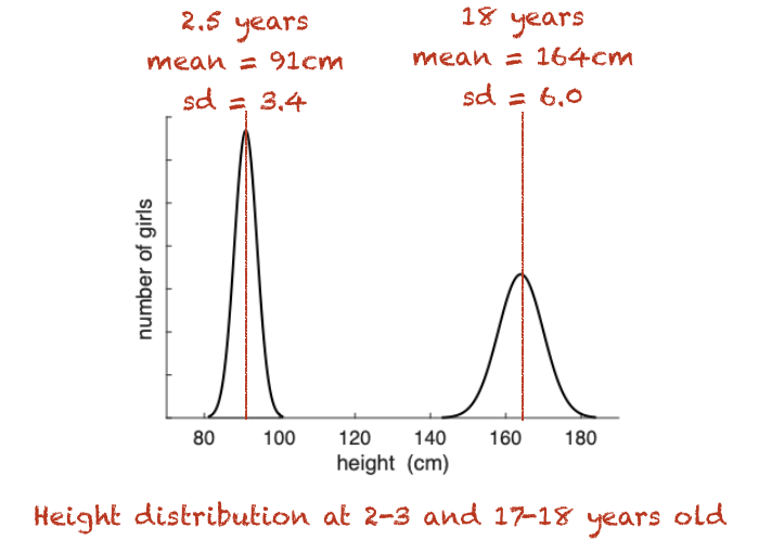
If some data (eg the heights of toddlers, or of adults) are normally distributed, that normal distribution can be summarized by two numbers or parameters:

• the mean of the distribution, \(\mu\)

  • in the example below, the mean height of 18-year-olds is unsurprisingly higher than the mean height for 2-year-olds)

• the standard deviation \(\sigma\)

  • in the example below, the spread of heights is larger for 18 year olds

Because we have the equation, once we know these two numbers we can estimate the full data distribution for heights (for example, I could tell you exactly how likely it is to be 95cm tall (to the nearest cm) as a toddler, or over 180cm as an adult woman)

Notation

When describing normally distribbuted data we sometimes use this notation:

\[ x \sim \mathcal{N}(164, 6.0^2) \]

To read this out loud we say:

“The heighht of adult women, \(x\), follows a Nomral with mean 164cm and standard deviation 6.0cm”

Note that there is some inconsistency in how different authors use this notation; some people specify the standard deviation and others the variance. To mminimie ambguity, I like to specify the standard deviation squared (ie the variance) as written above; it shhould be clear that \(6.0\) is the standard deviation and \(6.0^2\) is the variance

The Z-score

To standardize data by Z-scoring, we take two steps:

• subtract the mean (so the mean of the standardized dataset becomes zero)

• divide by the standard deviation (so the standard deviation of the standardized dataset becomes 1)

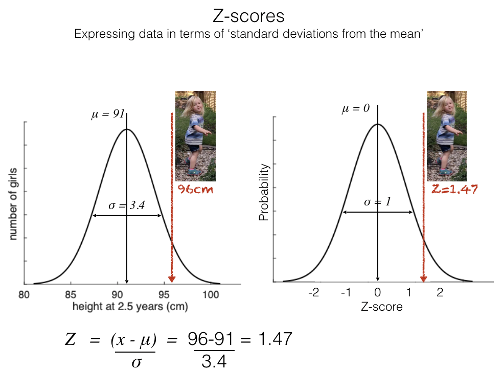
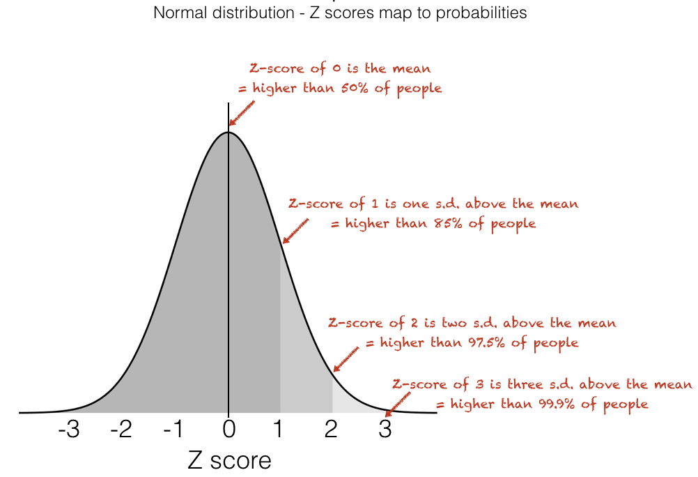
The result for normally distributed data is that the Z-scores translate directly into probabilities:

Equation

You can skip this subsection if you don’t fancy it

The equation of the bell curve is below. It has two parameters (numbers that vary between different normally distributed datasets): the mean \(\mu\) and the standard deviation \(\sigma\)

If we convert the data to Z-scores, we are standardizing the mean (to Zero) and sd (to 1), so the distribution of Z has no parameters that vary between datasets.

Looking closely at the simplifed form of the equation, we can see thhat the probability of a data value (or rather the corresponding Z-scores) is a function of the square of the Z-score, specifically \(e^{-Z^2}\).

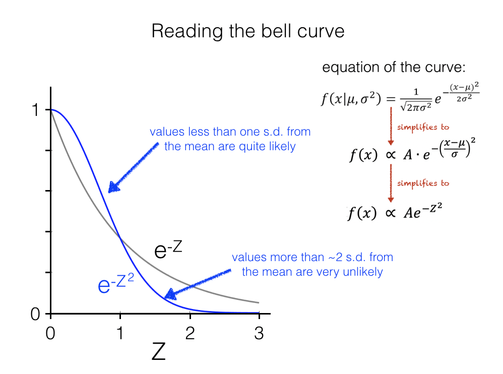
• The probability of observing a data value falls off for data values further from the mean under the Normal distribution

Comparing to the more familiar exponential decay curve \(e^{-Z}\) we see:

• Values less than one SD from the mean are quite likely (more likely under \(e^{-Z^2}\) than \(e^{-Z}\), because when \(Z<1\), then \(Z^2<Z\))

• Values more than 1 SD from the mean are increasingly unlikely (less likely under \(e^{-Z^2}\) than \(e^{-Z}\), because when \(Z>1\), then \(Z^2>Z\))

• As Z increases, the probability of observing a data value with that Z-score falls off rapidly, as \(Z^2 >> Z\) and \(e^{-Z^2}\) rapidly becomes tiny

  • This is what gives the normal distributions its thin tails

  • it means that if we try to fit a normal distribution to a dataset with an outlier, we end up estimating a very large standard deviation - because we can’t fit a normal that says one of our (say) 10 datapoints should occur only one in a million times (equivalent Z score of 4.75)

3.3.2. How do we know if data are normally distributed?

If we want to use a t-test we need to be confident that our data are approximately normally distributed

How can we know if this is the case?

For large samples we can plot a histogram and compare to the best-fitting normal. There are also statistical tests to determine whether data are normally distributed (but these are not covered here).

For smaller samples it is generally difficult to be confident that data are normally distributed. We can tell if data are strongly non normal by either:

• Plotting the data (although note even this isn’t very helpful for small samples)

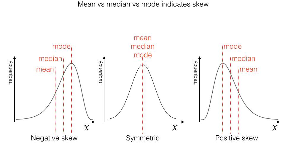
• Comparing the mean, median and mode to detect skew (normal data are symmetrical, not skewed)

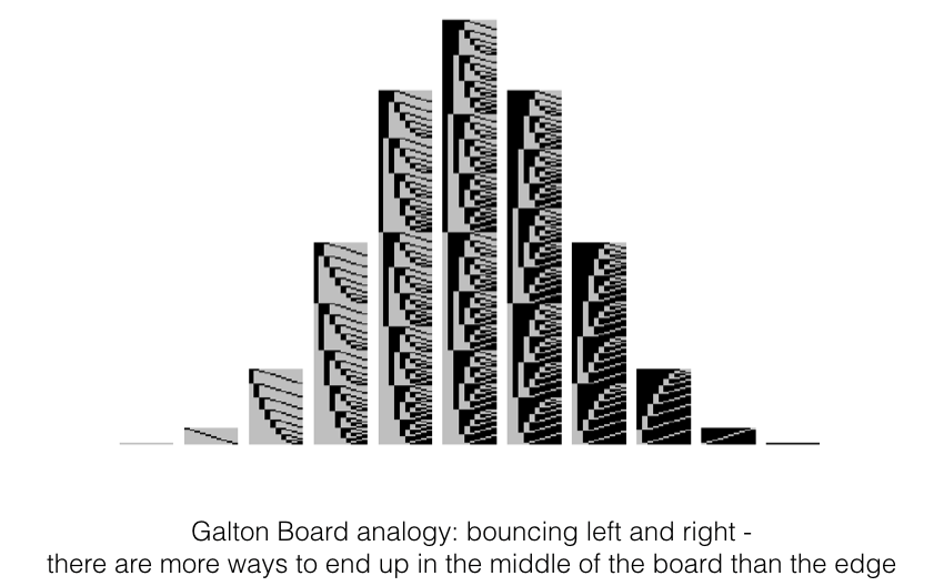
The main cases in which we could be confident that data in a small sample are normally distributed are cases in which there is a theoretical argument that the data should be normal, based on the Central Limit Theorem. Very roughly, the Central Limit Theorem explains that when a data value results from the summation of many independent influences (eg the influence of many genes on height, or the effect of a ball bouncing left- or right many times on a Galton board) the resulting data values follow a normal distribution.

The Central Limit Theorem will be covered in more detail later in the course.