4.10. Sample size and power

We have seen that the power of a test depends on the sample size, and a sample of a certain size is required for an effect to be detected with, say, 80% power.

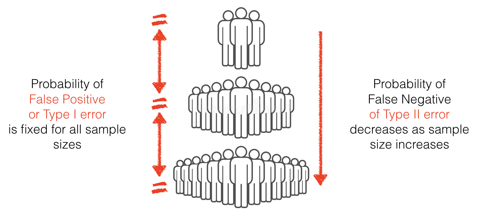
Most people will accept the intuition that increasing the sample size should make an experiment ‘better’, more reliable or more believable. However it is worth understanding that increasing the sample size primarily affects the proportion of false negatives NOT false positives. Hence sample size is relevant for the power of a test more than its \(p\)-value. This page explains why.

4.10.1. The proportion of false positives is fixed by design

In null hypothesis testing, the whole procedure is based on assuming \(\mathcal{H_o}\) is true:

• Choose an \(\alpha\) value

• Assume \(\mathcal{H_o}\) is true

we then

• Choose the critical value of the test statistic, so that the proportion of false positives \(\mathcal{H_o}\) is true) is \(\alpha\), eg 5%.

  • Reminder - the test statistic is a value like \(t\) or \(r\) on which a statistical test is performed

  • the critical value is the minimum value of that test statistic for which the test is significant, for a given \(n\)

This is equivalent to calculating the test statistic, finding the \(p\)-value and asking if \(p \lt \alpha\), but for this explanation it will be more helpful to think about it in terms of setting the critical value of the test statistic

So by definition the proportion of false positives, given the null is true, is fixed at 5% (or whatever \(\alpha\) is)

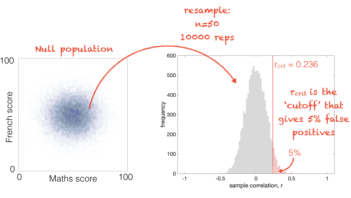
Example

Consider again the example from the Power by Simulation notebook:

I collect data on end-of year exam scores in Maths and French for 50 high school studehts. Then I calculate the correlation coefficient, Pearson’s \(r\), between Maths and French scores across my sample of \(n=50\) participants.

• \(\mathcal{H_0}\) Under the null hypothesis there is no correlation between maths scores and French scores

• \(\mathcal{H_a}\) Under the alternative hypothesis, there is a positive correlation

This is a one-tailed test, at the \(\alpha=0.05\) level

I can then work out the critical value of \(r\) using an equation as \(r_{crit}=0.236\).

• \(r_{crit}\) is the smallest value of \(r\) for which \(p<0.05\), for a given \(n\)

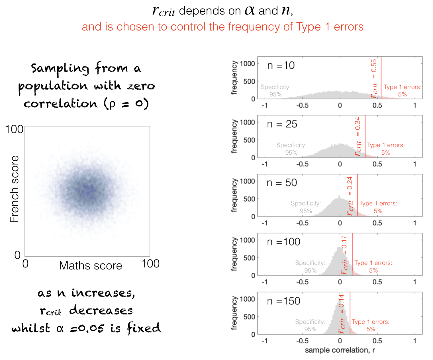
As \(n\) gets larger, \(r_{crit}\) gets smaller because the disribution of sample-values of \(r\) gets narrower - this can be seen in the following figure:

4.10.2. Proportion of false negatives is not fixed

In power analysis, the whole procedure is based on assuming \(\mathcal{H_a}\) is true

Assuming \(\mathcal{H_a}\) is true, we work out how often we would get false negative, based on the effect size, \(\alpha\)-value and \(n\).

One way to do this is simulating a correlated population and sampling from it, as we did in a previous notebook.

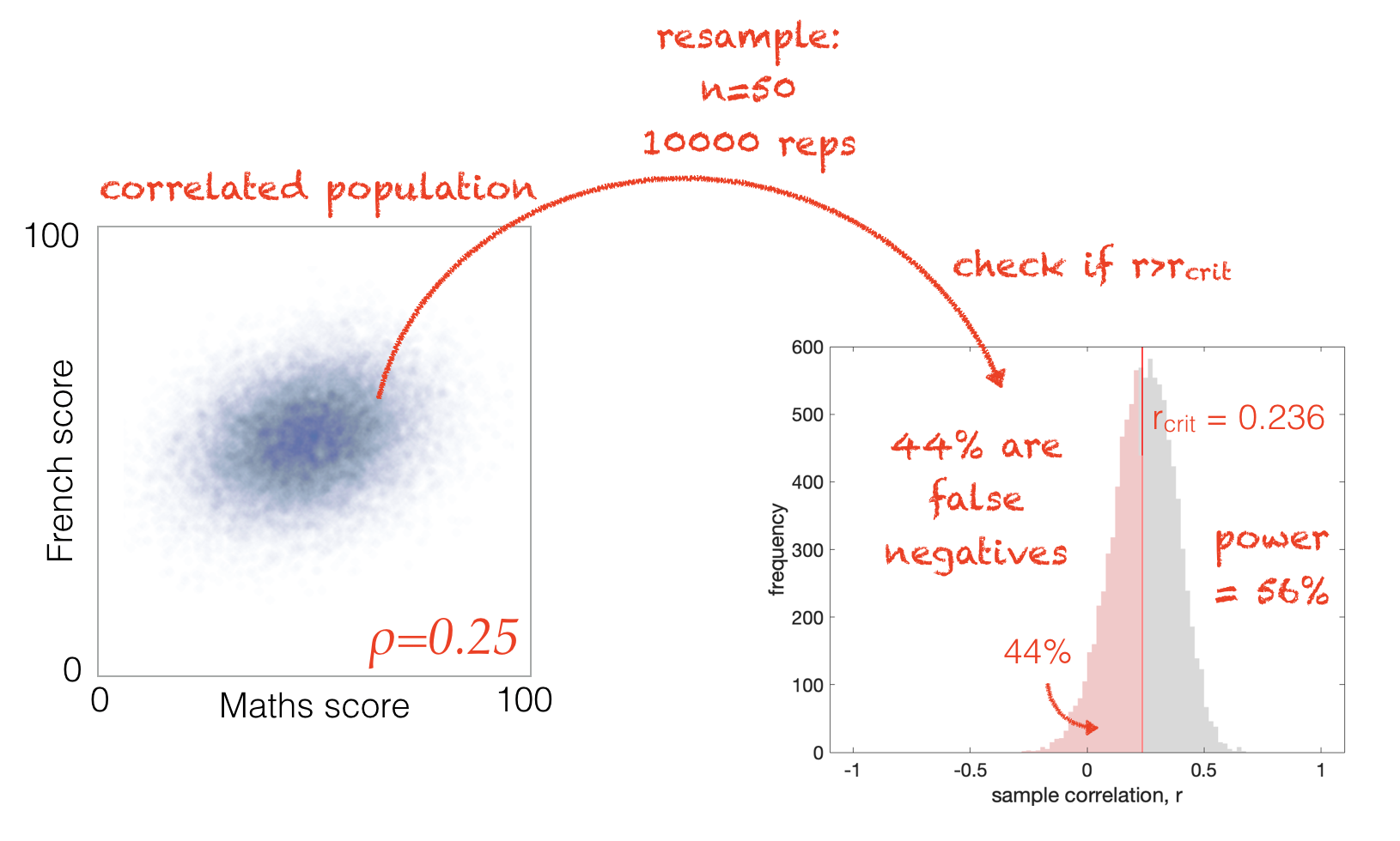
Note that \(r_{crit}\) is still the same \(r_{crit}\) determined based on the assumption that the null hypohthesis is true - it won’t move around based on what \(\rho\)is for this population (ie \(r_{crit}\) would be the same for versions of \(\mathcal{H_a}\) where \(\rho=0.1\) and \(\rho=0.9\), because \(r_{crit}\) is based on the assumption that \(\mathcal{H_o}\) is true and \(\rho=0\))

Looking at some samples drawn from a population with a fixed effect size (\(\rho=0.25\)), we can see that the distribution of sample correlation coefficients overlaps differently with \(r_{crit}\) depending on the sample size \(n\):

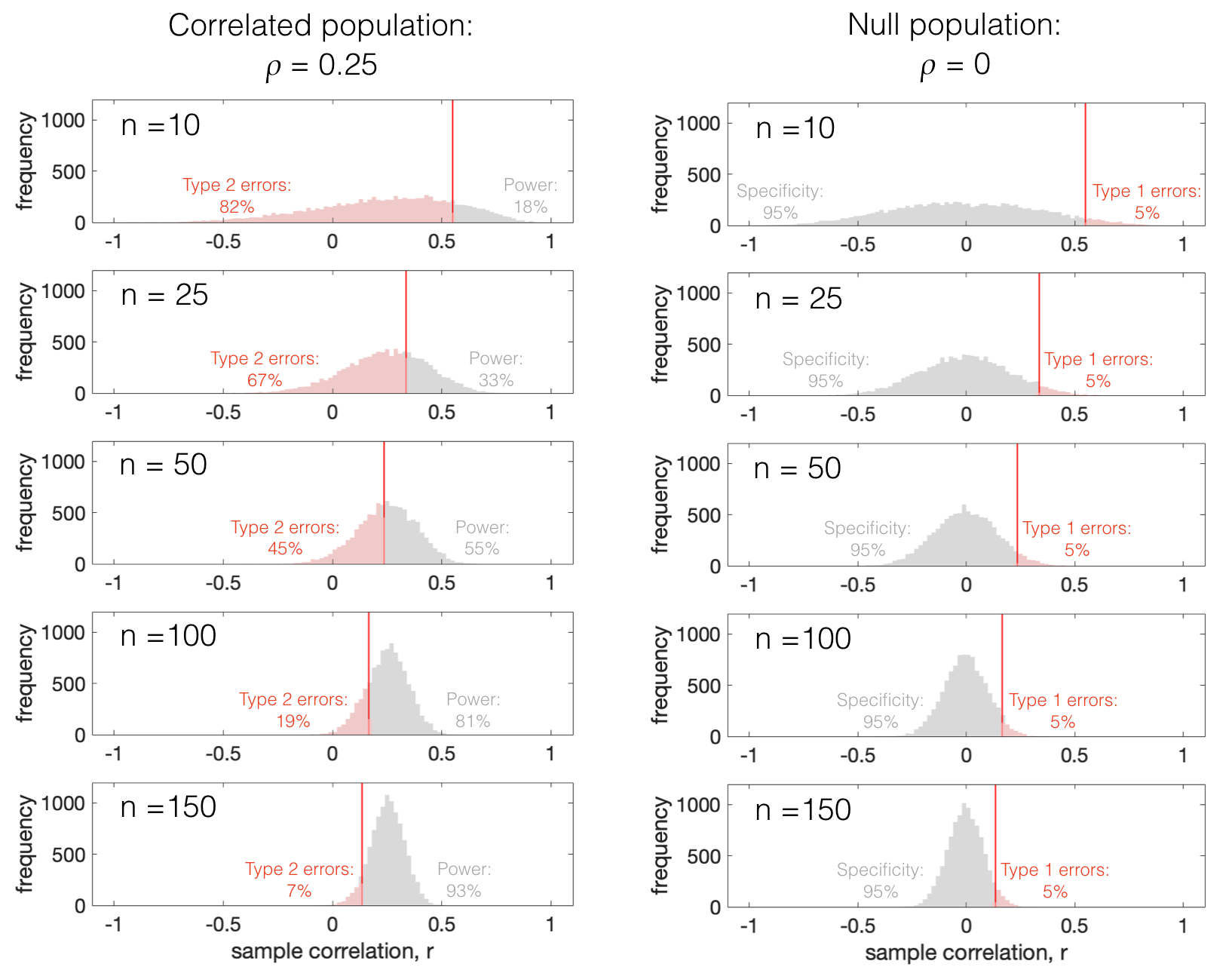
This is because of a “double whammy”:

• The distribution of \(r\) from the correlated population stays centred on \(r=\rho=0.25\) and gets tighter around that value

  • therefore the tail of the correlated distribution or \(r\) is pulled in towards \(\rho=0.25\) and away from zero

• \(r_{crit}\) retreats towards zero as the sample size increases

  • this is because as \(n\) increases, the null distribution (\(r\) values from the null population) gets tighter around \(r=0\), so r_{crit}$ moves towards zero therefore to maintain a tail of 5% of false positives

This interaction means that as \(n\) increases, fewer and fewer samples from the correlated population fall below \(r_{crit}\)

• ie there are fewer false negatives as \(n\) increases

4.10.3. Summary

• The proportion of false positives (if the null were true) is fixed regardless of \(n\)

• The proportion of false negatives increases as \(n\) gets smaller

4.10.4. Implications

Studies with insufficient power (because the sample size is too small) are unlikely to detect an effect even if there is one present in the underlying population. It is a waste of time and resources to carry our such a study.

Correlations, in particular, tend to need large sample sizes to achieve adequate power.