2.1. Kolmogorov Axioms

The Kolmomgorov Axioms (Kolmogorov 1933) formalize the definition of probability.

2.1.1. Events in probability theory

Axiom 1 concerns the probability of any event - an event could be a single event (rolling a 6), a compound event (tossing a coin and getting three heads in a row) or an observation that we wouldn’t in plain English, call an event at all (for example, that a person picked at random has blond hair).

Axioms 2 and 3 concern elementary events, which we can think of in terms of outcomes.

For example, if we roll a 6-sided dice twice, our elementary events could be defined in two ways:

• 36 possible sequences (1,2),(3,1),(6,6) etc - squares on the diagram below

• 11 possible total scores (2-12) - colours on the diagram below

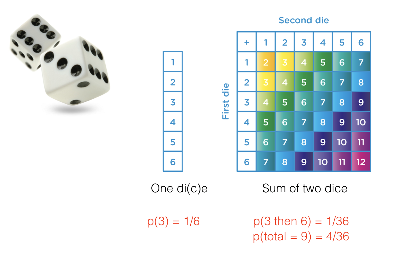
The definition of elementary events is the choice of the statistician and will reflect the statistical question you are trying to answer (“what is the probability of rolling (5,6)” is indeed a different question from “what is the probability of scoring 11”)

2.1.2. The Axioms

The Kolmogorov Algorithms summarize things you probably already knew about probability (and indeed these ideas were known before Kolmogorov formalized them mathematically in 1933).

A more mathematically correct account of the Kolmogorov Axioms can be found on Wikipedia.

Axiom 1

The probability of an event is a number beween 0 and 1

• Although sometimes it is more natural to express probabilities as a percentage.

• Take care not to mix up a probability of 0.1 (10%) and 0.1% !

Axiom 2

The sum of probabilities of all elementary events is 1

• Corollory - if all elementary events are equally likely, the probability of each elementary event is \(1/n\)

• For example, each possible outcome in a single diceroll has \(p=\frac{1}{6}\)

It is worth also considering the case in which there are no discrete elementary events. We describe the probability assocated with a continuous variable using a probability density function such as the one for a Normal distribution:

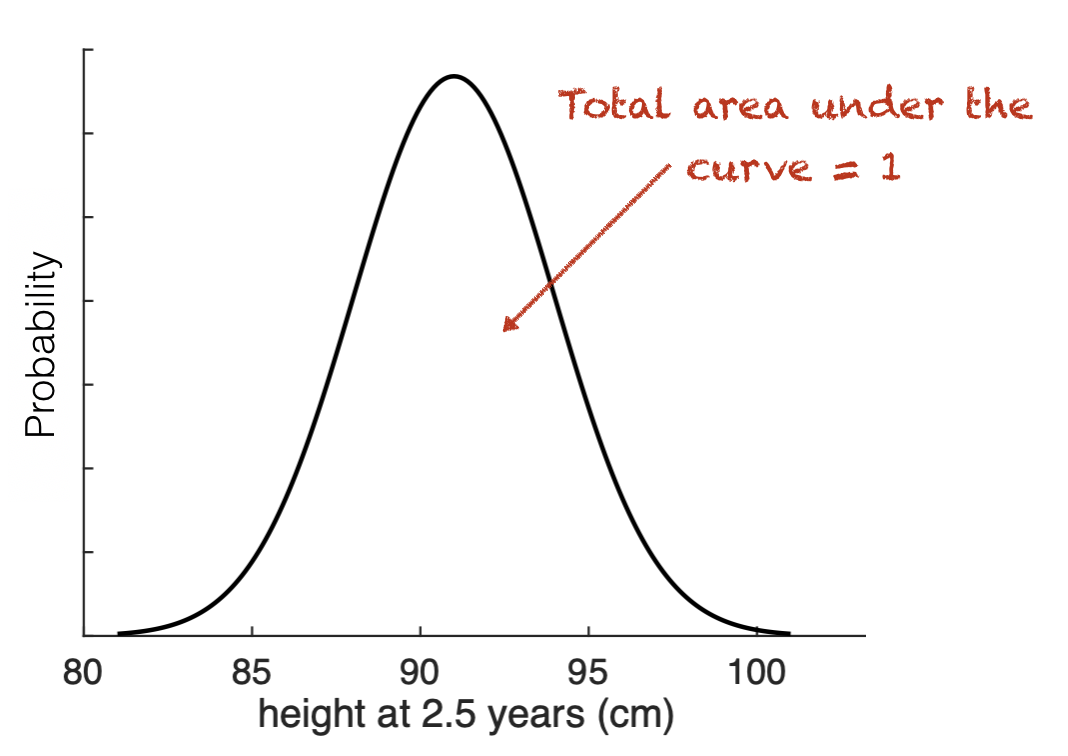
• The area under the curve of the Probability Density Function is 1

Axiom 3

The probability of some set of elementary elements is the sum of the individual probabilities

• For example, if we take the two sequences of two dicerolls that yield a total score of 11 (ie, (5,6) and (6,5)), the total probability is \(\frac{1}{36} + \frac{1}{36} = \frac{2}{36}\)

2.1.3. Events for a continuous variable

Thinking of probabilty over a continuous variable, where there are no discrete events, how do we define an event?

An example might be height; say heights for 2.5-year-old girls are normally distributed \(h \sim \mathcal{N}(91,3.4)\). An event is:

• That a child picked at random has a certain height

• the height must be defined as a range; probability is then the area within that range.

For example, what is the probability that a child’s height is 95cm, to the nearest cm (ie, height is in the range [94.5, 95.5)).

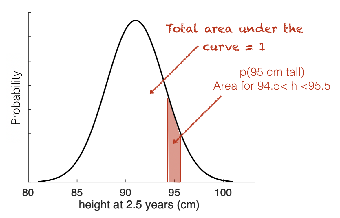
To do this in Python we could use stats.normal.cdf() twice:

• once to get the tail to the left of 95.5

• once to get the tail to the left of 94.5 and take it away, leaving the ‘strip’ from 94.5 to 95.5

stats.normal.cdf(95.5, 91, 3.5) - stats.normal.cdf(94.5, 91, 3.5)

Why can’t we simply calculate the probability of the height being exactly 95cm, by reading off the y-axis value associated with 95cm?

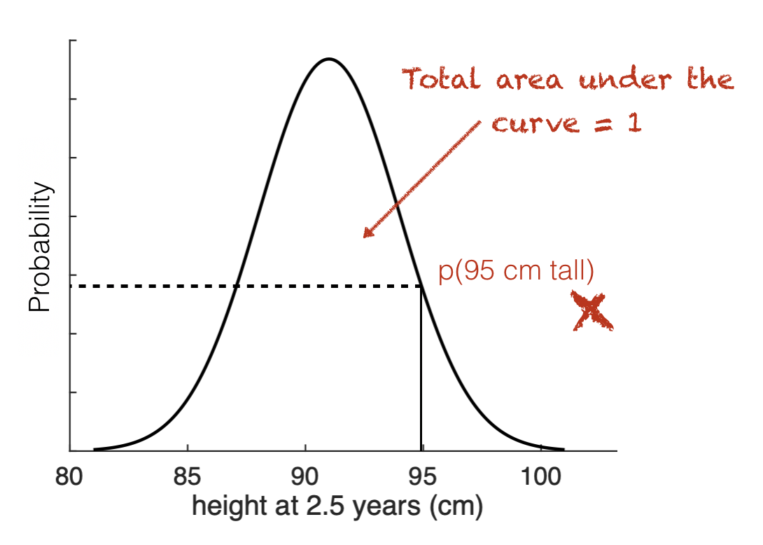
Because probability is defined as the area under the curve, and for a single point on the \(x\)-axis, rather than a range, there is no area.

When you think about it, what would exactly 95cm mean?

• if 95cm to the nearest cm, this is actually the range [94.5,95.5)

• If you mean 95.000000……. there will be fewer and fewer people matching this height as the specificity of the measurement gets narrower, til in the limit, no-one matches the height exactly.