
1.5. Permutation testing overview#
To evaluate the statistical significance of our test statistic, we need to know the null distribution of that test statistic, ie its distribution if the null hypothesis were true.
One way to do this is through permutation of the sample. This means shuffling around data in a way which shouldn’t matter (under the null hypothesis) but would matter if the alternative hypothesis were true.
Exactly which data we can shuffle depends on the type of test.
1.5.1. Independent samples, difference of means#
The simplest example is when we are interested in the difference of means between two independent groups, such as the heights of men and (unrelated) women.
In our example we had the following hypotheses:
\(\mathcal{H_o}\): Mean height of men = mean height of women
\(\mathcal{H_a}\): Mean height of men > mean height of women
Under the null hypothesis, everyone (men and women) is equally likely to be tall or short (there is a single distribution of heights). In this case, any difference in mean heights between the 25 men and 25 women in our sample is just random chance (all the tall people ended up in the men group by chance).
If the null hypothesis were true, the difference between men and women’s heights in our actual sample could just as well have arisen if we had allocating the labels ‘male’ and ‘female’ to 25 people each, regardless of their actual sex, and calculated the difference of means.
Using the computer, we can actually do this repeatedly to find the null distribution.
In shuffled data we retain features of the dataset that are independent of sex:
The overall distribution of heights (regardless of sex)
The sample sizes (25 in each group)
but we shuffle out the sex-based information:
randomly allocate the labels ‘Male’ and ‘Female’
1.5.2. Paired samples, difference of means#
Say we decide to use paired samples, comparing the heights of brothers with their sisters, to control for lifestyle and genetic factors that will be shared within families.
Our hypotheses remain the same:
\(\mathcal{H_o}\): Mean height of men = mean height of women
\(\mathcal{H_a}\): Mean height of men > mean height of women
Under the null hypothesis, each brother is equally likely to be taller or shorter than his own sister. Our test statistic is now the mean difference in height between each brother and his sister; this is not the same as the difference of means, because the difference between a brother and his own sister is more consistent than the difference between a man and a randomly chosen unrelated woman:
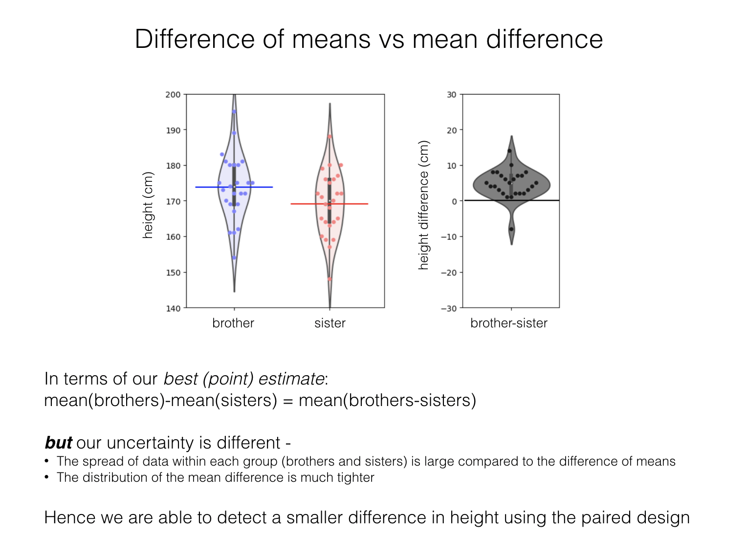
If the null hypothesis were true, the mean difference between each brother and his sister would have to have arisen by chance because the taller person in each family just happened to be the brother. In that case the difference could just as well have arisen from assigning the labels ‘brother’ and ‘sister’ randomly without each family regardless of each person’s actual sex.
Using the computer, we can actually do this repeatedly to find the null distribution - randomly flipping the labels ‘brother’ and ‘sister’ (or not flipping them) in each family.
In shuffled data we retain features of the dataset that are independent of sex:
The overall distribution of heights (regardless of sex)
The sample sizes (25 in each group)
The shared effect of family (correlation between brothers’ and sisters’ heights) - we do not move people between families
but we shuffle out the sex-based information:
randomly allocate the labels ‘Male’ and ‘Female’ within each family
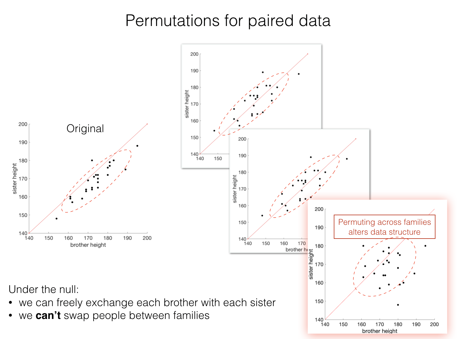
Note in the shuffled datasets that the correlation (effect of family) is retained but the data now lie around the line \(x=y\) (shown in red), whereas previously most of the data lay on one side of the line \(x=y\) indicating that brothers were consistently taller than their sisters. The final permutation (highlighted in red) breaks the family structure (not correct in this case - hopefuly you can see why from the figure).
1.5.3. Paired samples, correlation#
Say we are actually interested in the lifestyle and genetic factors that will be shared within families, and want to test whether brothers’ and sisters’ heights are correlated.
Our hypotheses are now:
\(\mathcal{H_o}\): The correlation between brothers’ and sisters’ heights is zero
\(\mathcal{H_a}\): The correlation between brothers’ and sisters’ heights is greater than zero
The observed correlation in our sample is \(r=0.9\)
Even if there was no family effect on height, it would sometimes happen that for 25 random families, the ones with the tallest brothers happen to be the ones with the tallest sisters. The question is how often a positive correlation as large as \(r=0.9\) would occur just due to chance if each brother was paired randomly with someone else’s sister.
Permutation#
The sample tells us several interesting things about the heights of men and women, regardless of family effects:
We retain some features of the height distributions:
Height is normally distributed within each sex
Men are taller than women
But we shuffle out the shared effects of family (the correlation):
tall brothers have tall sisters
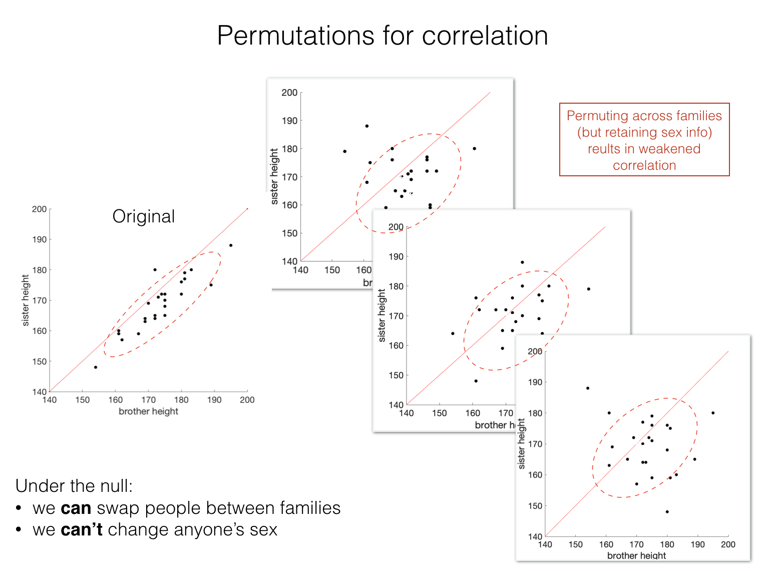
Note in the shuffled datasets that the correlation is lost, meaning the shuffled datasets are not ‘stretched out’ along the line \(x=y\) (shown in red). However, as in the original dataset, the shuffled datapoints mostly lie on one side of the line \(x=y\) indicating that brothers are (still) consistently taller than their sisters, because we didn’t ‘flip’ anyone’s sex in the shuffling process.
1.5.4. Summary#
We need to choose what to shuffle, and this is different for the three cases:
difference of means (indepedent samples)
difference of means (paired samples)
correlation
To decide what to shuffle we need to think about whihc datapoints are interchangeable under the null hypothesis.