4.3. False positives and False negatives

We can think of the hypothesis testing framework as a 2x2 grid of ‘reality’ vs ‘conclusions’

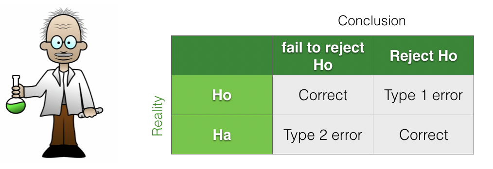
In this framework there are two ways of making an error:

• we reject the null hypothesis when it is in fact true (Type I error or false positive)

• we fail to rejct the null, when in fact the alternative hypothesis was true (Type II error or false negative)

As the terminology “Type I Error” and “Type II Error” is easy to mix up, I prefer the terms ‘false positive’ and ‘false negative’.

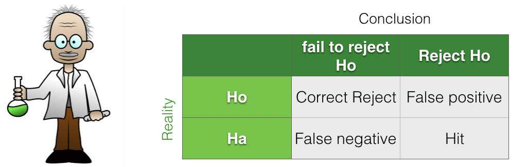
We can also classify the ‘correct’ cases as follows:

• Hits when \(\mathcal{H_a}\) is true, and we detect that (rejecting the null)

• Correct Rejects when \(\mathcal{H_o}\) is correct and we detect that (slightly confusingly, a ‘correct reject’ is when we correctly fail to rejct the null!)

4.3.1. Assuming \(\mathcal{H_o}\) vs assuming \(\mathcal{H_a}\)

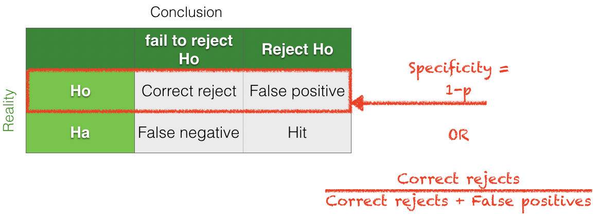
When calculating the \(p\)-value for a test, we assume \(\mathcal{H_o}\) is true and then work out the probabliity that we might reject \(\mathcal{H_o}\) due to chance. In other words, we are working on the basis of a certain state of reality, assuming \(\mathcal{H_o}\) is true.

Assuming \(\mathcal{H_o}\) is true:

• \(p\) is the proportion of false positives

• Specificity is \((1-p)\)

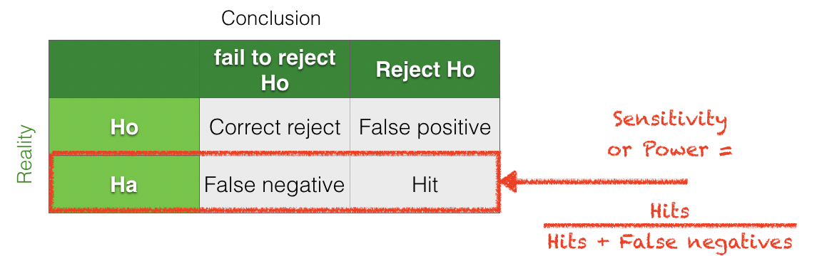
In contrast, in power analysis, we consider the alternative reality in which \(\mathcal{H_a}\) is true. Power is then theh probability that we correctly reject the null.

Assuming \(\mathcal{H_a}\) is true:

• Power is (1-proportion of false negatives)

• Sensitivity = power

Terminology

Because the terms sensitivity and specificity are easy to mix up, I prefer to talk about:

• the \(p\)-value of a test (which is 1-specificity) and

• the power of a test (equivalent to sensitivity).

4.3.2. Criminal analogy

It can help to think of an analogy to a criminal court:

• \(\mathcal{H_o}\): Everyone is innocent until proven guity

• \(\mathcal{H_a}\): He’s guilty, dammit!

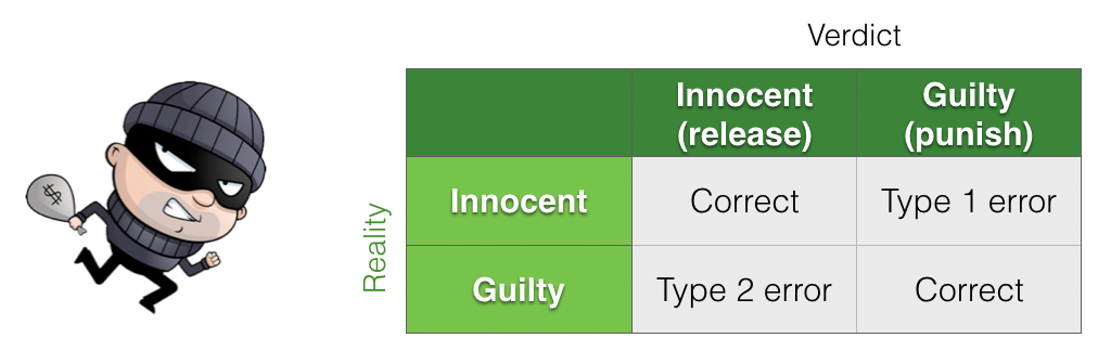
In this analogy:

• A Type I error (false positive) is a wrongful conviction

• A Type II error (false negative) is when the criminal gets away due to insufficient evidence

4.3.3. Insufficient evidence

The criminal analogy highlights the main cause of False Negatives (Type II errors) in scientific studies: insufficient evidence.

Often if we fail to get a significant result, when there is an underlying effect, it is because the sample size is too small.

This is because tests of statistical significance, and tests of statistical power, depend on three ingredients

• The effect size

• The sample size (\(n\))

• The \(\alpha\) value (the cut-off \(p\)-value for significance)

In general,

• The smaller the effect size, the larger the sample size neeed to detect it.

• The more stringent the \(\alpha\) value, the larger the sample needed to detect an effect of a given size

  • \(\alpha=0.001\) is more stringent than \(\alpha=0.01\) etc

The next pages will cover the definition of effect size.

4.3.4. Sample size primarily affects power, not \(p\)-value

Most people will accept the intuition that increasing the sample size should make an experiment ‘better’, more reliable or more believable. However it is worth understanding that increasing the sample size primarily affects the proportion of false negatives NOT false positives. Hence sample size is relevant for the power of a test more than its \(p\)-value. The reasons for this will be unpacked in the page Sample Size and Power in this chapter.