1.3. Mean, median and mode

First we consider measures of location, the mean, median and mode.

The mean, median and mode all give us an idea of the ‘average’ or ‘typical’ value of some measurement \(x\). However they differ in their properties and are therefore useful for different purposes.

Here is a video summarizing the conceptual differences between these measures.

1.3.1. Mean

Say I have a sample of \(n\) measurements, which we will call \(x_1, x_2 .... x_n\).

To calculate the mean of these measurements, I add up all the values in my sample and divide by \(n\):

\[ \bar{x} = \frac{\sum{x_i}}{n} \]

Here is an example where \(x_{1:7}\) are the heights of 7 people:

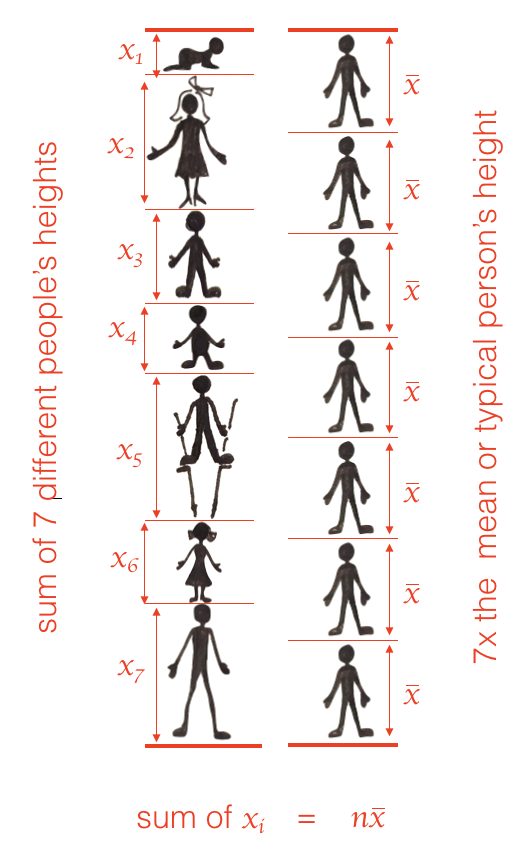
When visualized in this way, we can see a key property of the mean: the mean value, \(\bar{x}\), is a kind of “typical person” such that the mean height of a group of \(n\) people is the same as \(n\) times the “typical person’s” height \(n \bar{x}\).

This property of the mean implies that the mean tells us about the average or total value of a measurement for a large sample - for example, as described in the video above, if we know the mean length of a car, we can use this to predict the total length of a line of 100 cars. The median does not share this property

1.3.2. Median

The median is the middle ranked value or 50th centile of a dataset

To calculate the median I put all my measurements in order (I rank my datapoints) from the smallest (rank 1) to the largest (rank \(n\)). The median is the middle measurement (if \(n\) is odd), or the midpoint beween the middle two measurements (if \(n\) is even).

To obtain the median:

• Sort the values to obtain a list \(x_1, x_2, x_3 .... x_n\)

• Count the values to obtain \(n\)

• If \(n\) is odd, then the median is the middle value

• If \(n\) is even, the median is halfway between the middle two values

The median is the value which half of measurements lie above, and half below. For example if a child’s performance on a school exam is near the median, this means roughly half the children had higher scores and half had lower scores.

The median cannot be used to make predictions about the total measurement for a large group (for example, the length of a row of 100 cars) because, whilst it is the middle value, other values may not be symmetrically distributed about the median.

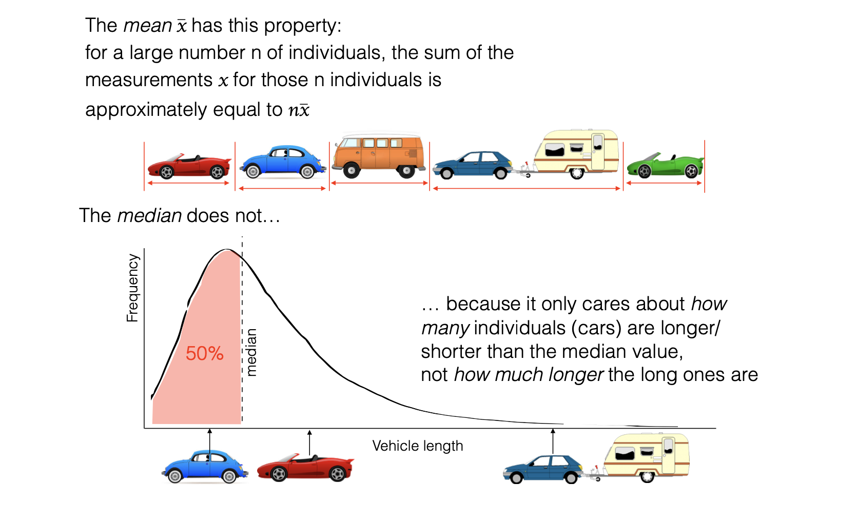
In a row of 100 vehicles as in the example above, there are equally many vehicles below the median length as above, but the very long examples (cars towing caravans etc) are not balanced out by equally extreme short vehicles - so the row of 100 vehicles will be more than 100x the median vehicle length.

Centiles

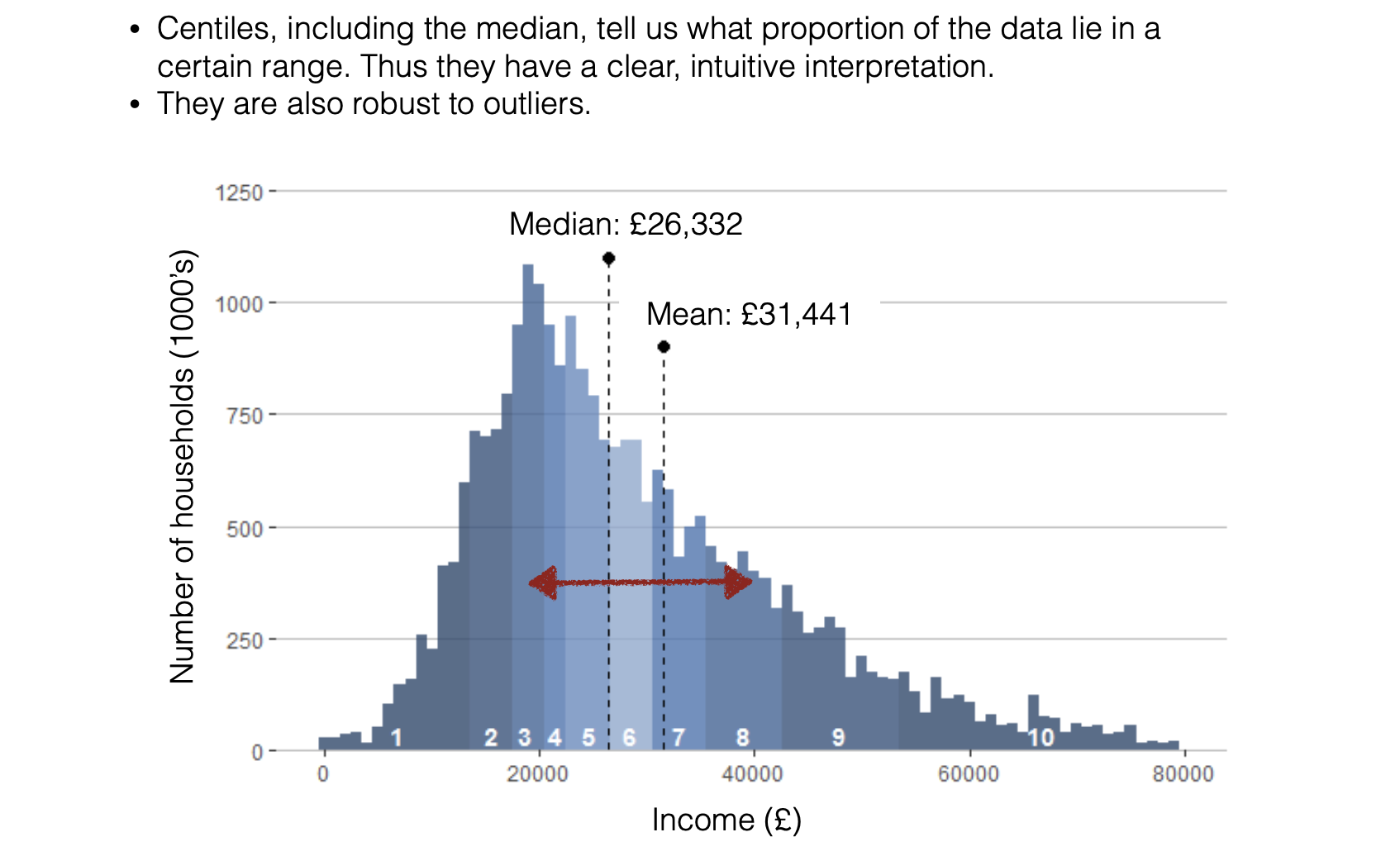
A generalization of the median is the idea of centiles of a distribution - for example the 90th centile is a value exceeded by only 10% of measurements. This is easily interpreted: if a child’s height is ‘on the 90th centile’ that means that they are taller than 90% of children their age, and will look tall in a crowd of same-age children.

Centiles, including the median, are therefore useful for telling us rather directly where an individual datapoint stands in relation to a distribution.

Relatedly, centiles including the median can be used determining values that ‘cut-off’ a certain percentage of individuals - for example what percentage of people earn over £100,000 per year, or how long would a parking space need to be to accommodate 99% of cars?

1.3.3. Mode

The mode is the peak of the distribution.

There are two cases in which we would be particularly interested in the mode:

1. For categorical variables - for example asking which party received the most votes in an election, or which type of pet is most popular. For categorical variables, the mean and median don’t really apply

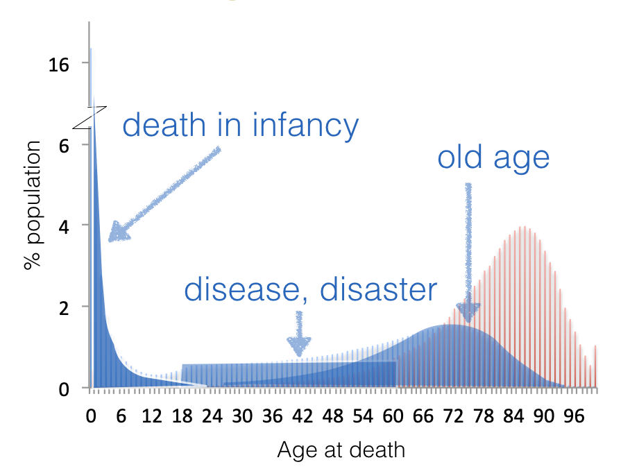
2. Describing the shape of a distribution - for example, we saw in the lecture that the “age at death” distribution from pre-industrial times had multiple modes.