1.3. Hypothesis testing concepts

This week we introduce Null hypothesis testing, the framework in which most statistical tests are carried out.

1.3.1. Defining null and alternative hypotheses

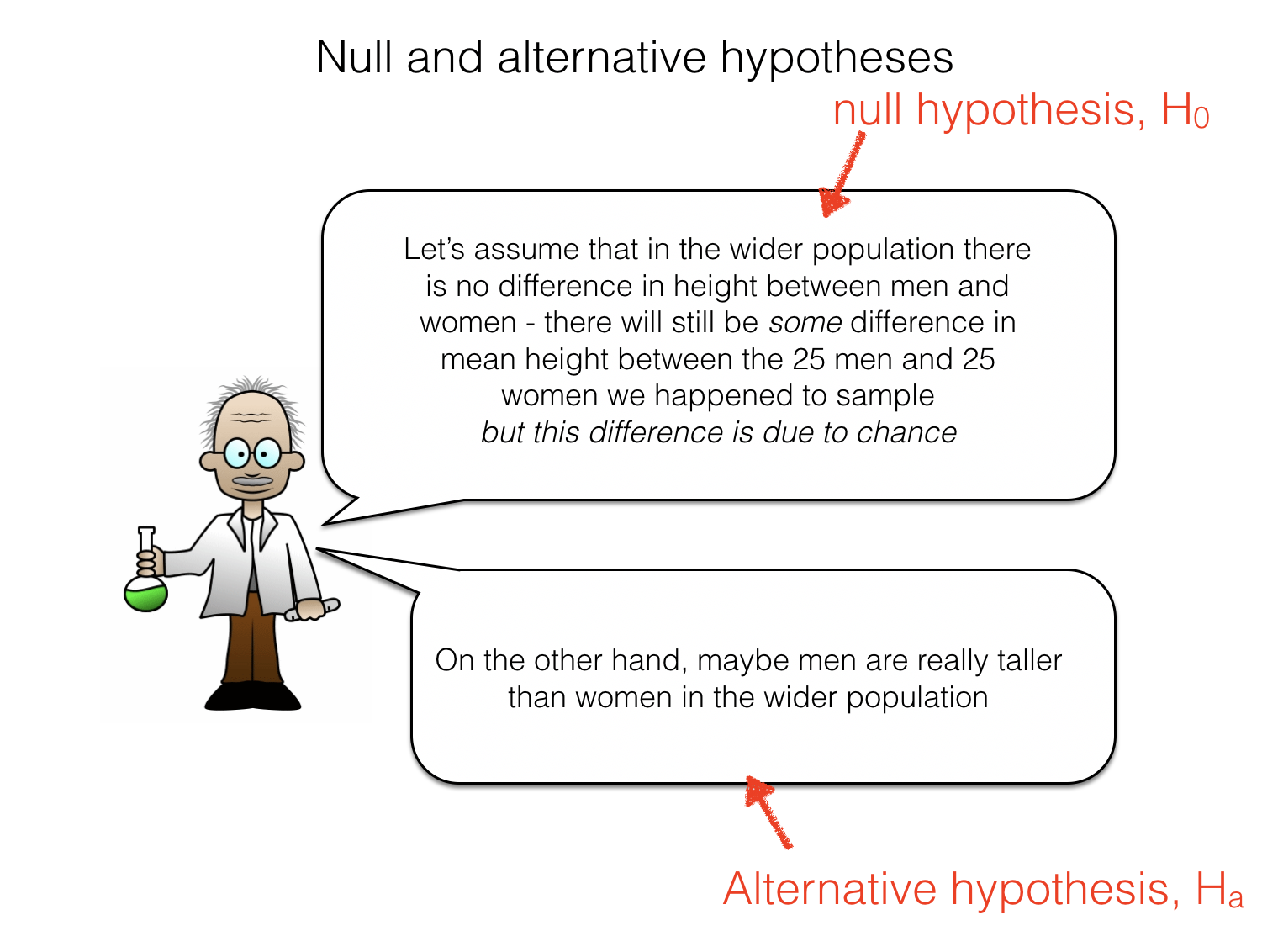
When testing for a statistical effect in data (such as a difference in means between groups), we specify a null hypothesis and an alternative hypothesis

• The null hypothesis \(\mathcal{H_o}\) describes a situation where the statistical effect of interest is absent

• The alternative hypothesis \(\mathcal{H_a}\) describes a situation where the statistical effect of interest is present

For example, a researcher hypothesises that men are taller than women. The null and alternative hypotheses are as follows:

• \(\mathcal{H_o}\): Mean height of men = mean height of women

• \(\mathcal{H_a}\): Mean height of men > mean height of women

Note that the alternative hypothesis specifies the direction of the effect of interest. In this case we have a strong expectation that men are taller than women. We could have stated an alternative hypothesis proposing the opposite direction of effect:

• \(\mathcal{H_o}\): Mean height of men = mean height of women

• \(\mathcal{H_a}\): Mean height of men < mean height of women

of a neutral (two-tailed) alternative hypothesis

• \(\mathcal{H_o}\): Mean height of men = mean height of women

• \(\mathcal{H_a}\): Mean height of men ~= mean height of women

note the symbols ~= and != simply mean ‘is not equal to’

1.3.2. Test statistic

The test statistic is a descriptive statstic calculated for our sample, whose significance we are evaluating.

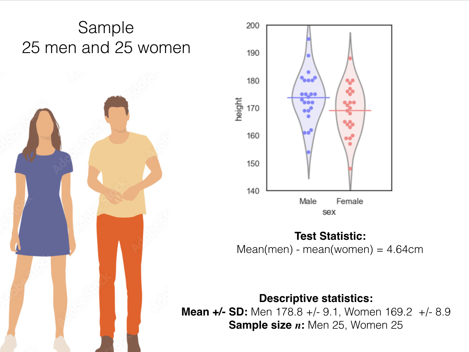
In this case, the test statistic is the difference in mean heights between men and women. Say we measure the heights of 25 men and 25 women; the test statistic is:

difference of means(men - women) = mean(men’s heights) - mean(women’s heights)

or ‘the difference of means’ for short.

Some other examples of test statistics are:

• the mean difference (between paired data points, such as height of brothers and sisters)

• the mean of a single group (tested against zero or some other reference value, eg is the IQ of Oxford students significantly higher than the average value in the general population, 100?)

• a correlation coefficient sich as Pearson’s or Spearman’s \(r\)

Further examples that we will meet next week:

• the \(t\) statistic for a difference of means, mean difference or Pearson’s \(r\)

• the rank sum and sign rank test statistics, U or R and T.

1.3.3. Descriptive statistics

You should report relevant descriptive statistics for your test. Which descriptive statistics are appropriate depends on the test:

• for the \(t\)-test (next week!) you need the mean(s), standard deviation(s) and group size(s)

  • exactly which ones depends on whether you have independent or paired samples, \(n\)

• for the rank-based tests (next week!), you need the median(s) and inter-quartile range(s), and group size(s), \(n\)

• for the permutation tests this week, you need the mean(s) of the groups, the standard deviations(s) and the group size(s), \(n\)

In this example we have the following:

1.3.4. Assume the null is true

We then try to work out the probability that the observed test statistic could have occurred even if the null was true

To do this we procede to assume the null hypothesis is true, and ask:

** if we had many many samples of data of the same size as our real/measured sample, how often would we get a value of the test statistic as extreme as the one we actually observed **

1.3.5. Null distribution

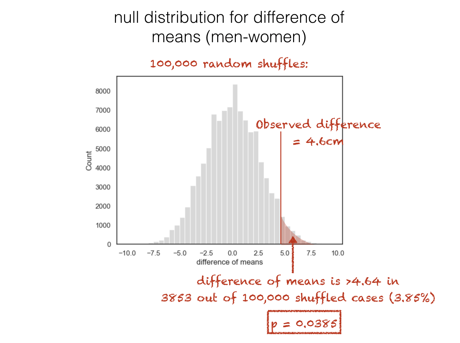
We therefore calculate the null distribution of the test statistic (the distribution of values of that test statistic we would get, if indeed we had many many samples of data of the same size as our real/measured sample)

This week will will calculate the null by permutation, but we will meet other methods next week.

1.3.6. \(p\)-value

The probability that the observed value of the test statistic could have occurred if the null hypothesis were true is sometimes called the \(p\)-value.

In the example above, the \(p\)-value associated with the observed difference of means is 0.038 or 3.8%

It means that, even if there was no underlying difference in height between men and women, if we repeated the experiment (pick 25 random men and 25 random women and measure their height) many times, we would expect to get a difference in mean heights as large as the one observed (4.64cm), 3.8% of the time.

Of course, the idea of repeating the experiment (pick 25 random men and 25 random women and measure their height) lots of times is exacly what the permutation process is designed to simulate.

1.3.7. \(\alpha\)-value

The result is usually considered statistically significant if is smaller than some predetermined level, known as the \(\alpha\) value.

Usually \(\alpha = 0.05\) or \(\alpha = 0.01\) is used, so the result is statistically significant if \(p < 0.05\) or \(p < 0.01\).

1.3.8. Reject or fail to reject the null

The logic of null hypothesis testing is that if the result is statistically significant, it was unlikely to have occurred if the null was true. Therefore if the result is statistically significant we can reject the null hypothesis.

If the results is not statistically signiciant, all we can say is that we fail to reject the null hypothesis. Why can’t we say we “accept the null”? The reason is that we are assuming the null hypothesis is true and trying to see if there is evidence against it. Therefore, the conclusion should be in terms of rejecting the null.