1.4. One- and two-tailed tests

In our height example, our researcher hypothesised that men are taller than women. The null and alternative hypotheses were as follows:

• \(\mathcal{H_o}\): Mean height of men = mean height of women

• \(\mathcal{H_a}\): Mean height of men > mean height of women

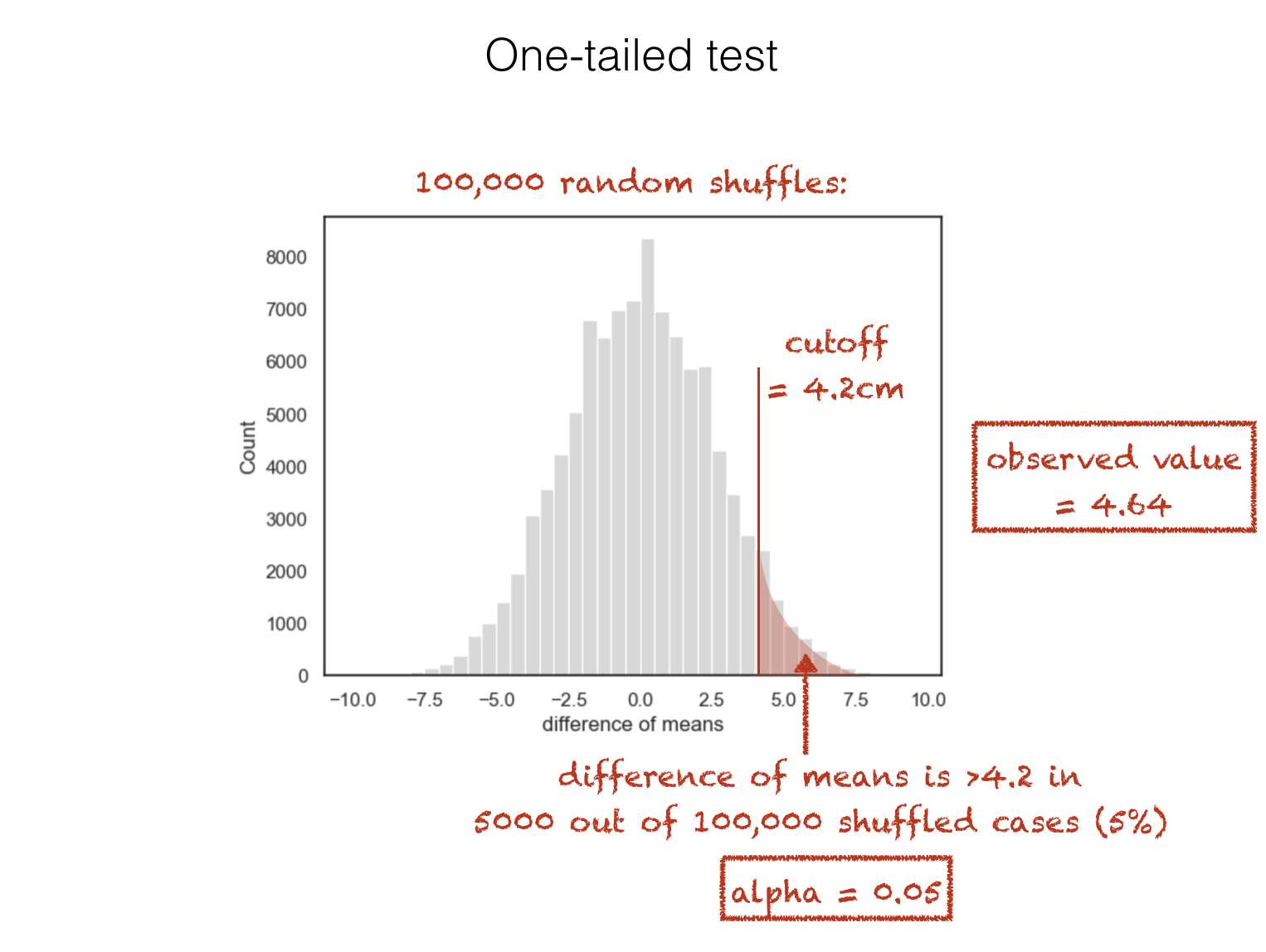
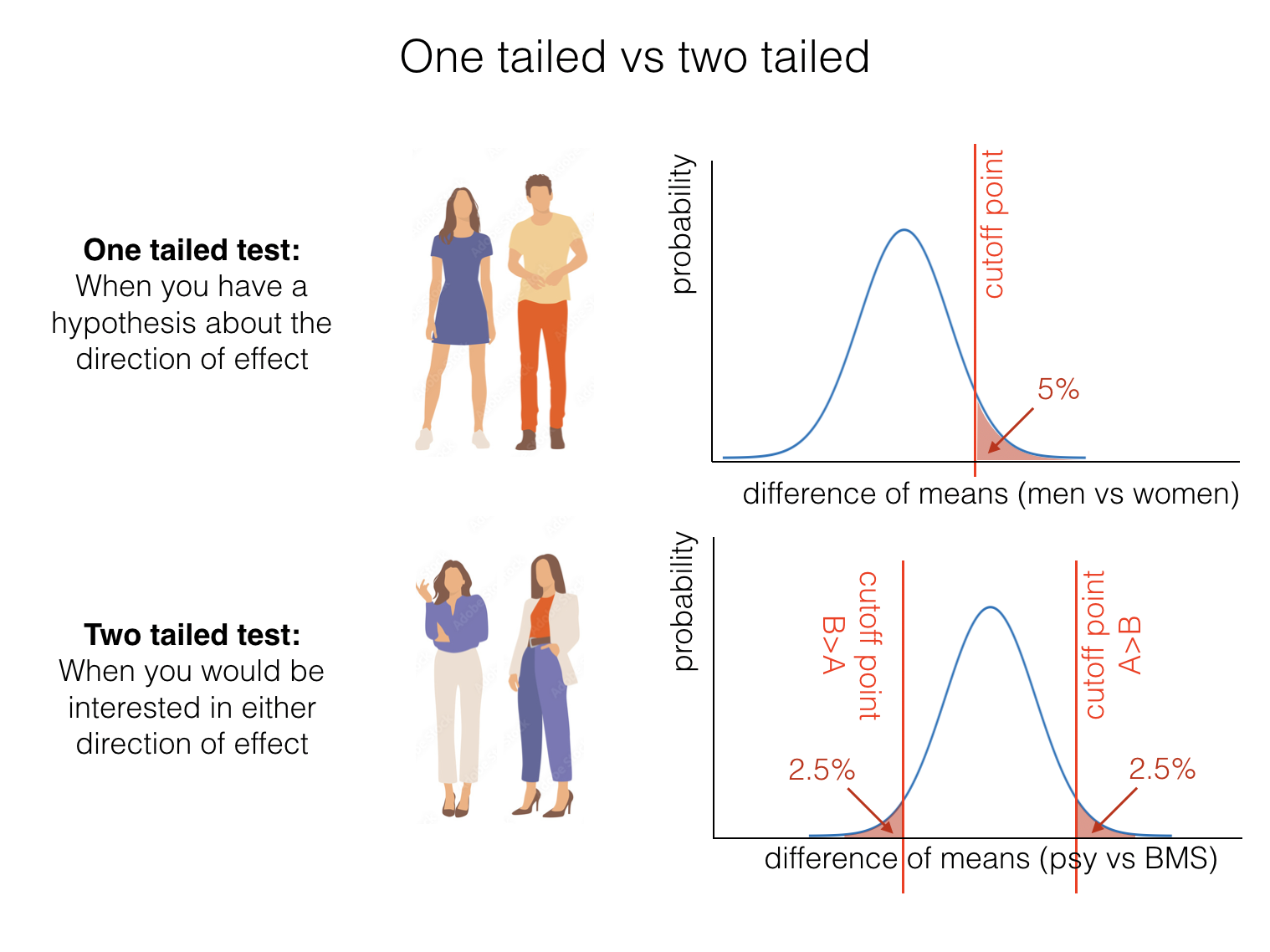
The above is a one-tailed test because the alternative hypothesis specifies the direction of the effect of interest. In this case we have a strong expectation that men are taller than women.

In terms of the null distribution, this means we will consider our observed difference of means significant if it falls in one of the tails of the null distribution (the tail containing cases where the mean height of men is much greater than the mean height of women; specifically if \(\alpha=0.05\) then the ‘tail’ contains the top 5% of values for the difference of means in shuffled data):

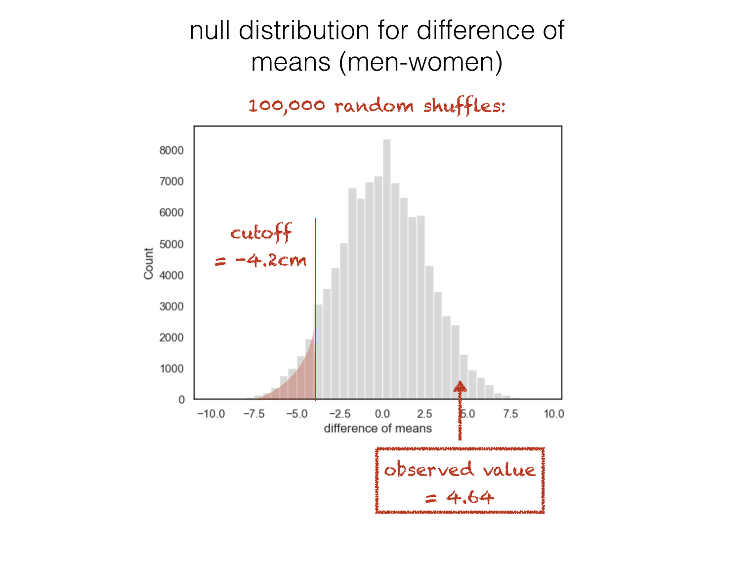
We could have stated an alternative hypothesis proposing the opposite direction of effect:

• \(\mathcal{H_o}\): Mean height of men = mean height of women

• \(\mathcal{H_a}\): Mean height of men < mean height of women

… in which case we would have considered the result significant only if it fell in the other tail (the tail containing cases where the mean height of men is much less than the mean height of women):

1.4.1. Two tailed test

In some cases, we may wish to remain neutral about the direction of the expected effect; in this case we specify a two-tailed alternative hypothesis:

• \(\mathcal{H_o}\): Mean height of men = mean height of women

• \(\mathcal{H_a}\): Mean height of men ~= mean height of women

note the symbols ~= and != simply mean ‘is not equal to’

In the case of men’s vs. women’s heights this may seem odd (since we know from experience that men are taller than women). However there are many scenarios in which we wouldn’t have a strong expectation about the direction of the effect - for example, if we compared the heights of Psychology and Biomedical Sciences students.

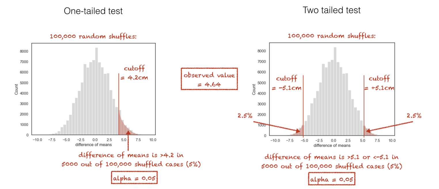
When we run a two-tailed test, we would consider our result (difference of means) significant if it fell in either tail of the null distribution. This means that we need to set the cut-off value for significance such that the area in both tails adds up to the \(\alpha\) value; so if we are testing at the 5% level, \(\alpha = 0.5\), the cutoff value in each tail needs to be such that each of the tails contains 2.5% of cases:

This means that the difference of means needed to achieve statstical significance in a two-tailed test is higher or more stringent than for a one-tailed test. In our height example, the result would be significant for a one-tailed test but not a two-tailed test:

For this reason it may be tempting to “cheat” and claim that you had a hypothesis beforehand about the direction of the effect (when you really didn’t), but to do so would, of course, not be statistically valid.

1.4.2. Python

When running statistical tests with scipy.stats you will need to specify whether the test is one- or two-tailed using an argument, such as alternative='greater'. The default (what happens if you don’t specify the argument) is generally two-tailed.