2.4. Event combinations

In this section we look at some statistical ideas concerning sequences or combinations of events, especially

• The complement

• Joint probability

• Marginal probability

• Conditional probability

• Combined probability

• Mutually Exclusive events

NOTE -

These examples use hair and eye colour, based on probabilities in the UK.

2.4.1. Complement: \(E^c\)

The complement of an event is simply that event not happening.

For example, say I randomly select a person on the street:

• let \(H\) be the event that a randomly selected person has blond hair

• \(H^c\) is the event that a randomly selected person does not have blond hair

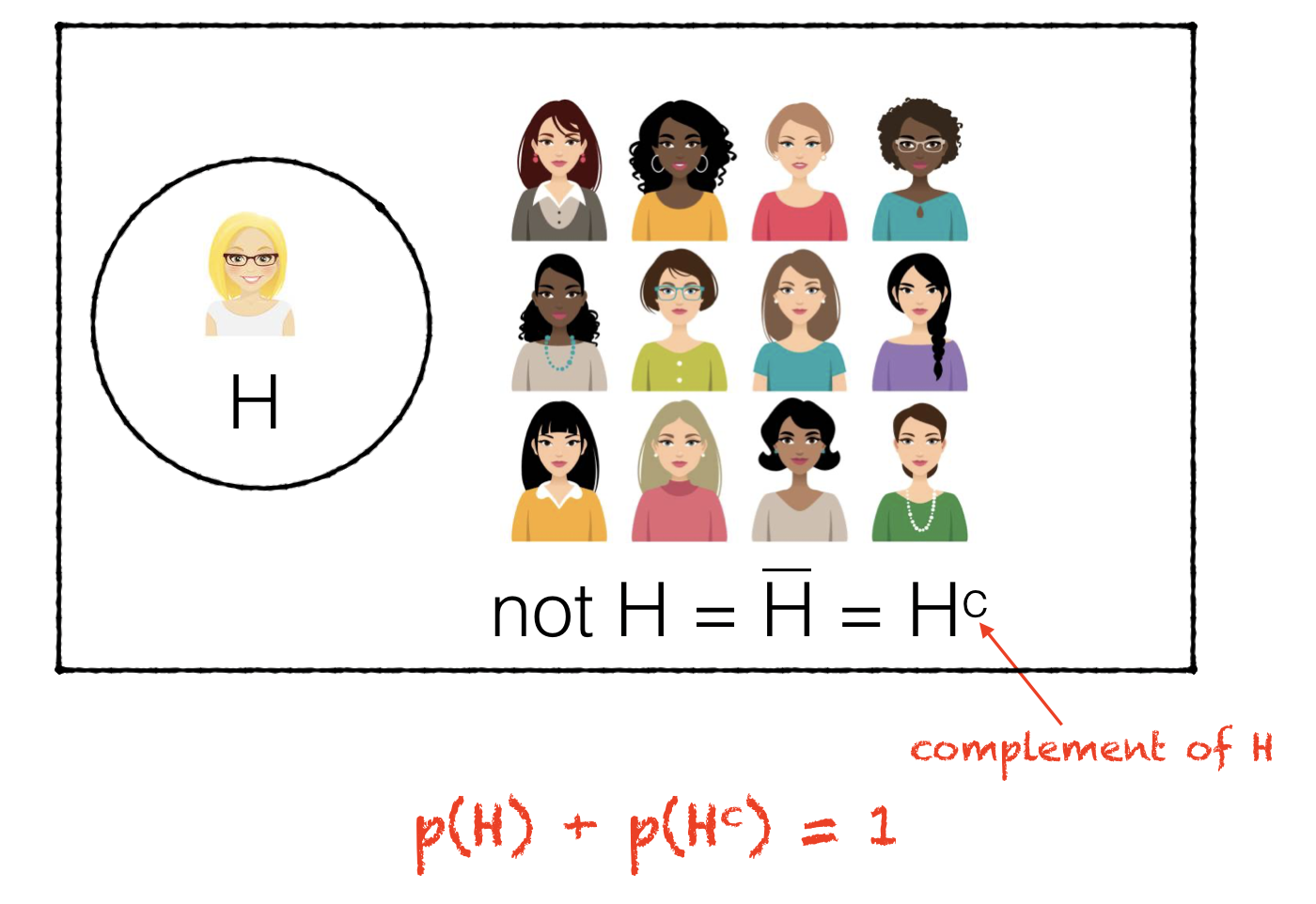
The probability of an event and its complement must add up to 1 (since any time the event doesn’t happen, the complement does, and vice versa)

• hence \(H^c\) is defined as ‘not blond hair’ rather than, for example, ‘brown hair’, as there will be some people who do not have blond or brown hair

NOTE- this is an example of Kolmogorov’s second axiom!

2.4.2. Marginal probability \(p(A)\)

The marginal probability of an event A is the total probability of A occurring, regardless of which other events (e.g. B, C) may occur.

The marginal probability of A is simply written \(p(A)\)

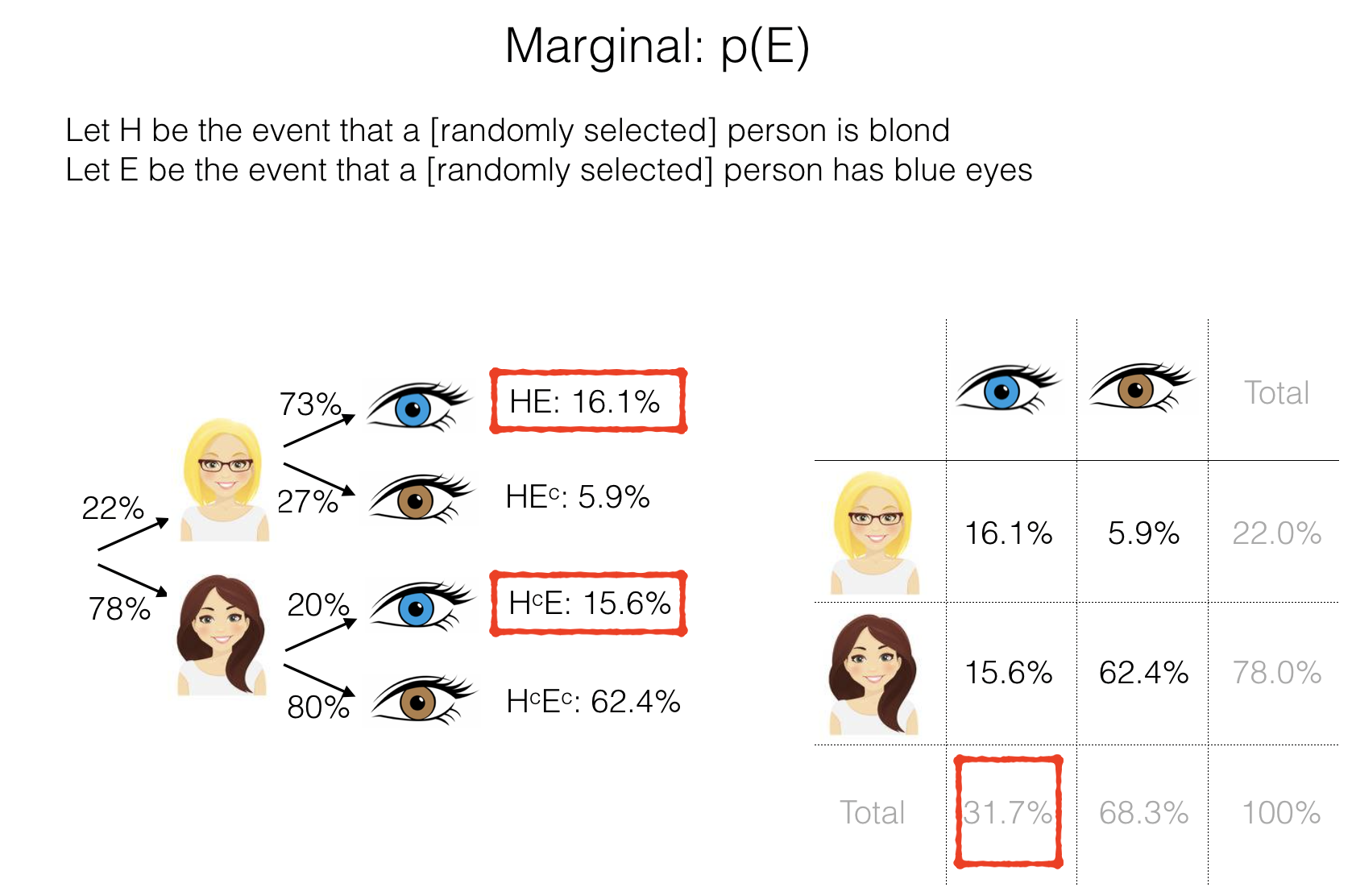
Marginal probability is perhaps most clearly illustrated in the contingency table - the marginal probability of blue eyes is the sum of all the cells in the blue eyes column. The marginal probability is therefore written in the ‘column total’ cell at the bottom of the blue-eyes column.

In the probability tree, the mariginal is the sum of multiple brances (all the branches that include a blue eye)

2.4.3. Conditional probability \(p(A|B)\)

The conditional probability is the probability of one event, conditional on another event having happened/ being the case.

For example, the conditional probability of a person having blue eyes given that we know they have blond hair, \(p(E|H)\) = 0.73%, which is quite different to the overall or marginal probability of having blue eyes \(p(E)\) = 32%.

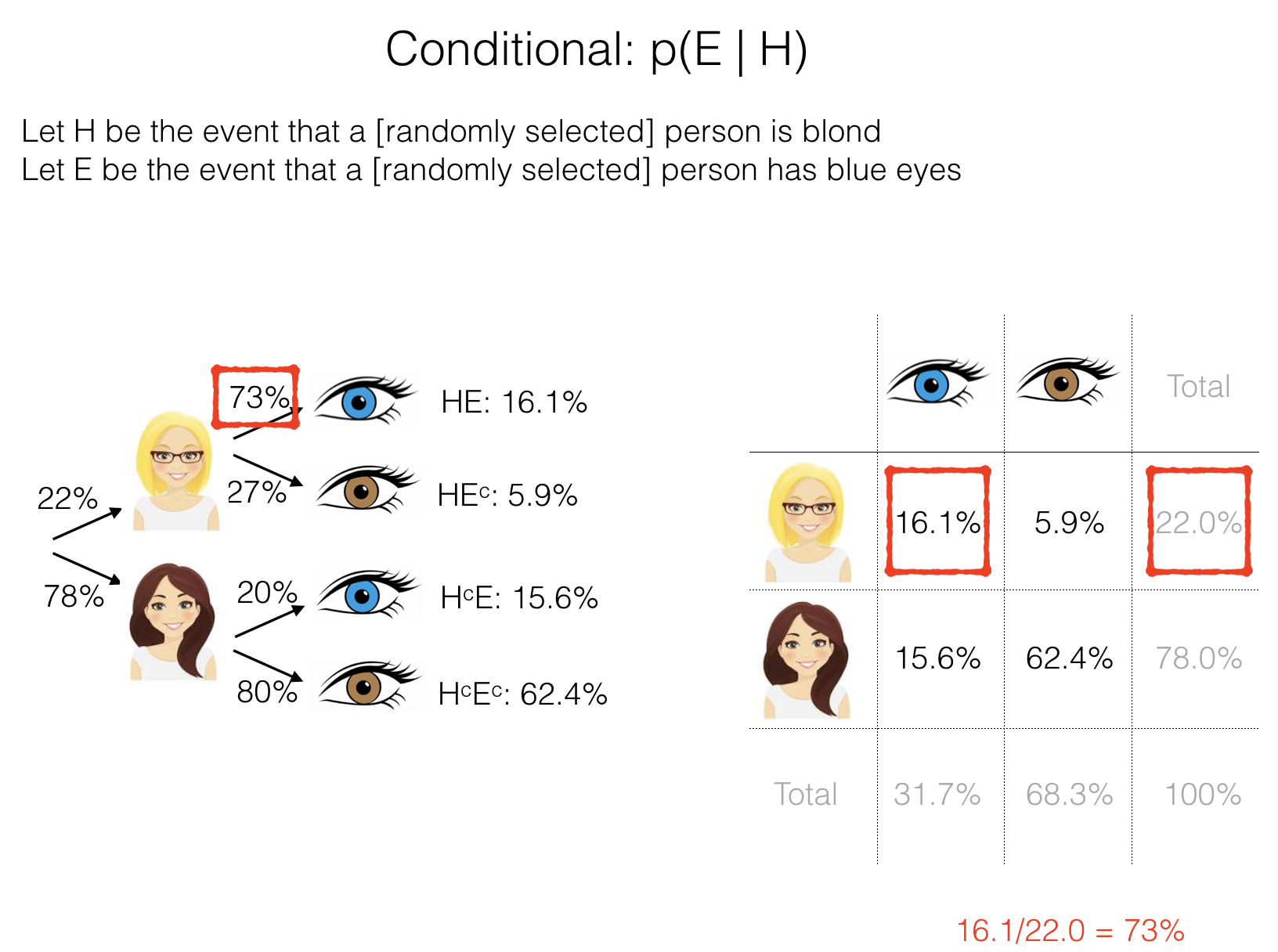
To work out the conditional probability based on the contingency table, we need to divide the probability in the cell for \(E\) and \(H\) (\(p(E \cap H)\) - see ‘joint probability’ below) by the row total for \(p(H)\).

Conditional probability is much more clearly visualized from the probabilities on the second set of branches in the probability tree (where we see that \(p(E|H)\) = 73% is quite different from \(p(E|H^c)\) = 20%.

The difference in conditional probabilities is proof that \(E\) and \(H\) are not independent**:

• If two events \(A\) and \(B\) are independent, \(p(A|B) = p(A|B^c)\) and \(p(B|A) = p(B|A^c)\)

2.4.4. Joint probability \(p(A \cap B)\)

The joint probability of events A and B is the probability that they both happen.

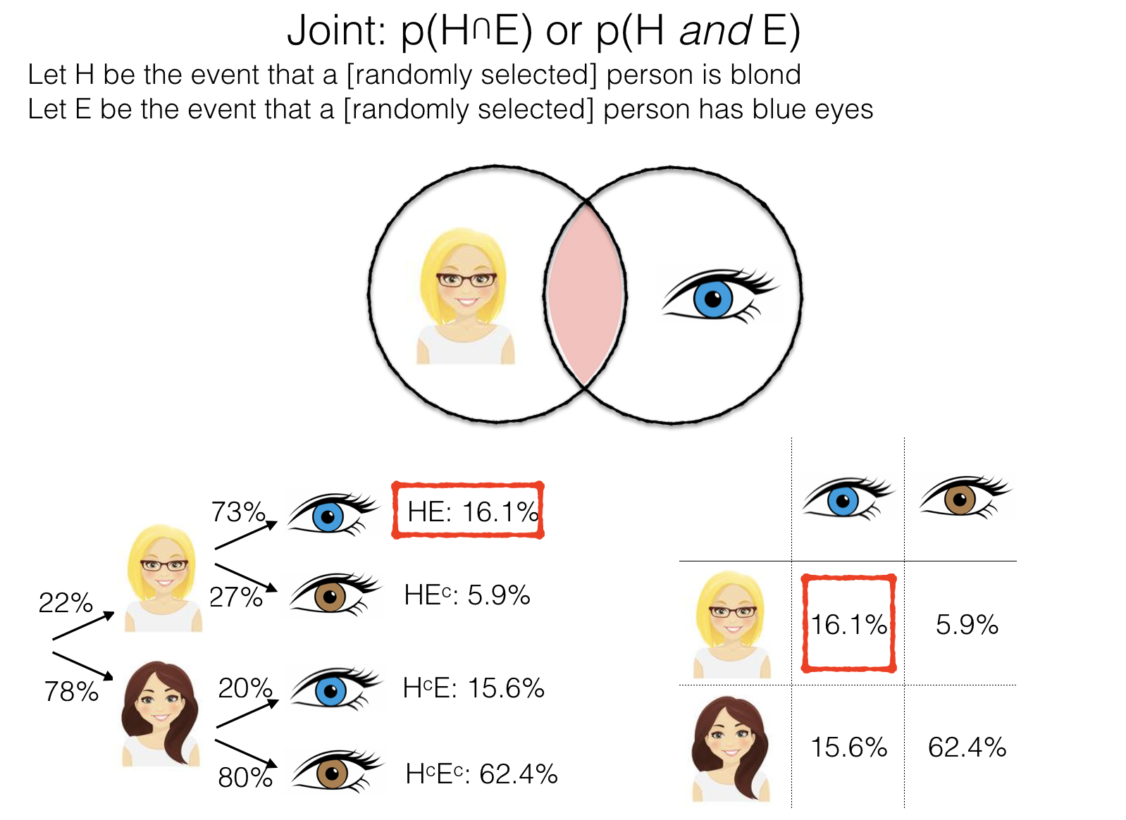
The joint probability is sometimes called the intersection of A and B - which makes sense looking at the Venn diagram above.

In this example, the joint probability is the probability of reaching the end of a single branch in the probability tree or a single cell in the contingency table

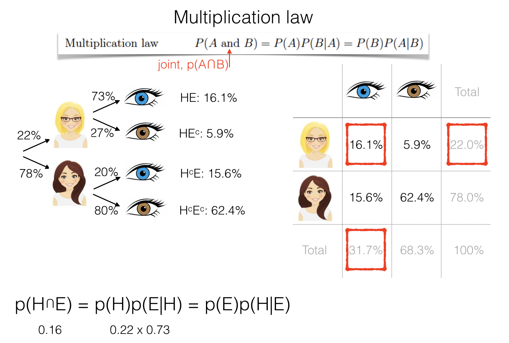
Multiplication law

You may be familiar with the idea that the probability of two independent events (for example, getting a six on two consecutive dice rolls) is the product of the individual probabilities:

\[p(6,6) = p(6) \times p(6) = \frac{1}{6} \times \frac{1}{6}\]

of more generally,

\[p(A \cap B) = p(A) \times p(B)\]

However, if events are not independent, the probability of the second event depends on the outcome of the first, and the equation above does not hold.

For example, what is the probability that a randomly chosen person has blond hair and blue eyes? We work our way along the relevant branches of the probability tree

First we check the hair:

• Let H be the event that a person has blond hair. 22% of people have blond hair, so p(H)=0.22.

Then we check the eyes.

• Let E be the event that a person has blue eyes. p(E)=0.32

However, we already know that this person has blond hair (we are already in the ‘blond’ branch of the probability tree. So we need something slightly different

• (E|H) is the event that a person with blond hair has blue eyes p(E|H)=0.72

To obtain the joint probability we need to use the multplication law:

\[p(E \cap H) = p(E|H) \times p(H)\]

2.4.5. Combined probability \(p(A \cup B)\)

The situation where eiter A or B occurs is sometimes called the Union of A and B and is written \(A \cup B\).

The idea of a union of events is most obviously useful when thinking of combining different cases of the same variable - for example

• Let \(A*\) be the event that a randomly chosen person got an A* on an exam

• Let \(A\) be the event that a randomly chosen person got an A on an exam

The \(p(A* \cup A)\) is the probability that a randomly chosen person got an A or A*.

When two events are mutually exclusive (cannot happen be the case) the probability of their union is obtained by adding up the individual probabilities.

For example, since an individual could obtain only one grade on a given exam, \(A^*\) and \(A\) are mututally exclusive and \(p(A^* \cup A) = p(A^*) + p(A)\)

We may sometimes want to know the combined probability of non-mutually-exclusive events; for example, what is the probability that someone obtained a grade combination of (A*/A) or higher, over two exams?

To solve this we invoke the Addition Law

Addition Law

The addition law is:

\[p(A \cup B) = p(A) + p(B) - p(A \cap B)\]

To understand this equation, think about our exam grades example:

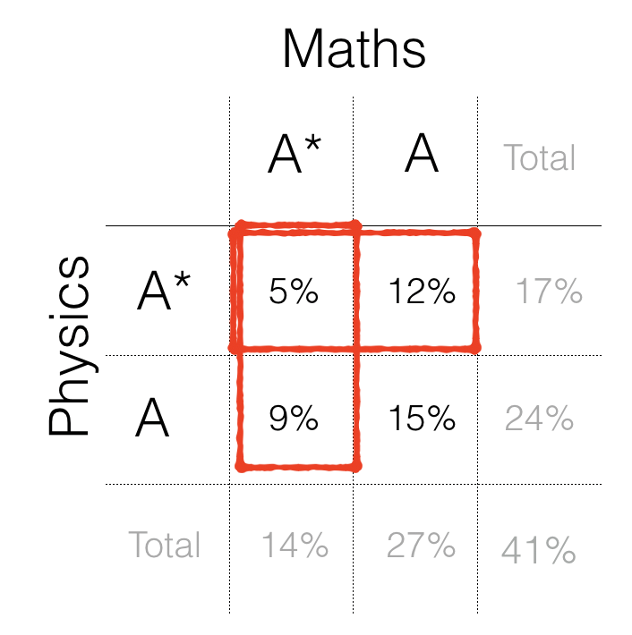
If we tried to work out the probability that someone has a grade combination of (A*/A) or higher, we could try to add up the areas represented by the two shaded rectangles:

• the probability that they have an A* in physics (given that they got an A or A* in maths): 17%

• the probability that they have an A* in maths (given that they got an A or A* in physics): 14%

…giving a (wrong!) total of 31%

This approach is wrong because it would count the people who got (A*/A*) twice (the double-shaded region in the contingency table) - so we need to subtract the 5% probability of (A*/A*). This gives the answer of 26%, which is what we would get if we added up the three cells meeting the criterion “A*/A or higher” directly: 5%+12%+9% = 26%.

Note that whilst this may seem obvious looking at the contingency table, it is an easy mistake to make when probabilities are presented in other ways.