
1.1. The Binomial Distribution#
Consider the following situations:
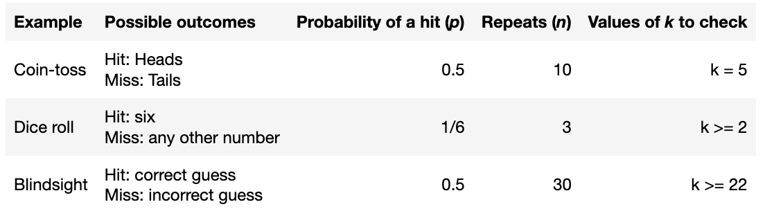
a fair coin is tossed 10 times. How likely is it that we obtain exactly 5 heads?
a fair six sided dice is rolled 3 times. How likely is it that we obtain two or more sixes?
a blind man guesses whether a symbol on a screen is an X or an O. How likely is it that he guesses correctly at least 22 out of 30 times?
In each case there is an event with two possible outcomes.
One outcome (the one we are looking for) is designated as a “hit” whilst the other is called a “miss”.
The probability of a hit is a fixed value (\(p\))
The event is repeated a certain number of times (\(n\)) and we count the number of times (\(k\)) one of the outcomes (the “hit”) occurs
In each case we can ask:
What is the probability of obtaining \(k\) (or at least \(k\)) hits out of \(n\) trials, given that the probability of a hit on any given trial is \(p\)?
The probability of each value of \(k\) is given by the binomial distribution
1.1.1. Tasks for this week#
Conceptual material is covered in the lecture. In addition to the live lecture, you can find lecture videos on Canvas.
Please work through the guided exercises in this section (everything except the page labelled “Tutorial Exercises”) in advance of the computer-based tutorial session.
To complete the guided exercises you will need to either:
open the pages in Google Colab (simply click the Colab button on each page), or
download them as Jupyter Notbooks to your own computer and work with them locally (eg in JupyterLab)
If you find something difficult or have questions, you can discuss with your tutor in the computer-based tutoral session.
This week is particularly heavy on conceptual material, so please do discuss the guided exercises and tutorial exercises with your tutor to make sure you understand